Yang Xiao-Xia, Daamen Winnie, Paul Hoogendoorn Serge, Dong Hai-Rong, Yao Xiu-Ming. Dynamic feature analysis in bidirectional pedestrian flows. Chinese Physics B, 2016, 25(2): 028901
Permissions
Dynamic feature analysis in bidirectional pedestrian flows
Yang Xiao-Xia1, Daamen Winnie2, Paul Hoogendoorn Serge2, Dong Hai-Rong1, †, , Yao Xiu-Ming3
State Key Laboratory of Rail Traffic Control and Safety, Beijing Jiaotong University, Beijing 100044, China
Department of Transport and Planning, Faculty of Civil Engineering and Geosciences, Delft University of Technology, Delft 2628 CN, Netherlands
School of Electronic and Information Engineering, Beijing Jiaotong University, Beijing 100044, China
Project supported jointly by the National Natural Science Foundation of China (Grant No. 61233001) and the Fundamental Research Funds for Central Universities of China (Grant No. 2013JBZ007).
Abstract
Abstract
Analysis of dynamic features of pedestrian flows is one of the most exciting topics in pedestrian dynamics. This paper focuses on the effect of homogeneity and heterogeneity in three parameters of the social force model, namely desired velocity, reaction time, and body size, on the moving dynamics of bidirectional pedestrian flows in the corridors. The speed and its deviation in free flows are investigated. Simulation results show that the homogeneous higher desired speed which is less than a critical threshold, shorter reaction time or smaller body size results in higher speed of flows. The free dynamics is more sensitive to the heterogeneity in desired speed than that in reaction time or in body size. In particular, an inner lane formation is observed in normal lanes. Furthermore, the breakdown probability and the start time of breakdown are focused on. This study reveals that the sizes of homogeneous desired speed, reaction time or body size play more important roles in affecting the breakdown than the heterogeneities in these three parameters do.
The movement of pedestrian flows is an extremely complex procedure. Since the early 1970s, the study on pedestrian dynamics has attracted the attention of researchers. The modeling methods have been emerging in order to study pedestrian behaviors in normal conditions during evacuation.[1–5]
Generally, pedestrian models can be divided into three categories: macroscopic, mesoscopic, and microscopic models. Some good overviews on pedestrian models are presented in Refs. [6] and [7]. Pedestrian models play an important role in understanding the dynamic features of pedestrian flows which are characterized by different self-organization behaviors. Zipper effect,[8] lane formation in the bidirectional flow,[9] strips in the crossing flow,[10] and other self-organization phenomena[11] have already been investigated using various pedestrian models or walker experiments. Moreover, pedestrian models are also used to assess designs and operations of building constructions such as stations, airports, and stadiums.[12] The social force model[13] is considered as the reference model in this paper. One reason is that the social force model as a microscopic model can qualitatively represent self-organization behaviors such as arching and lane formation.[13] Another reason is that the social force model considers both physical factors and motivational factors, which makes the simulated pedestrians more realistic.[14]
In recent studies, the bidirectional flow as one of the typical pedestrian flows has attracted more and more attention of scientists because of its various dynamic movement features. Pedestrians in the bidirectional flow are spontaneously organized in lanes with a uniform walking direction if the density of pedestrians is high enough.[15] According to Ref. [16], there are three phases in the bidirectional flow: the freely moving phase, the coexisting phase, and the uniformly jamming phase. Additionally, phase transition from coexisting phase to congestion occurs with an increase in entrance density in the bidirectional flow.[17] Congestion starts when pedestrians cannot maintain speeds in their desired directions, which may result in a temporary or total standstill which implies breakdown.[18] However, we are still not clear whether breakdown will occur after congestion starts, or when this breakdown occurs. Besides, the bidirectional flow usually contains pedestrians in heterogeneity.[19] Some people may walk faster because of their preference or due to some urgent matters, others may walk slower because of gender, age, disability, and some people may have better abilities to regulate their velocities according to the real-time situation of the pedestrian flow. The movement state, however, is more sensitive to which types of pedestrian flows is also unclear.
On the basis of previous studies, the dynamic phenomena of both free flows and congestion flows with homogeneity or heterogeneity are mainly focused on in this paper. The mean speed of the free flow and the fluctuations in speed are investigated in order to reflect the effects of homogeneity and heterogeneity in different parameters of the social force model on free flow dynamics. By comparing the values of the mean speeds and their standard deviations, we can obtain that the free flow dynamics is more sensitive to which parameter of the social force model with homogeneity or heterogeneity. Besides, some observed walking behaviors in this paper further contribute to better understanding different free flows. Moreover, the performances of congestion flows reflected by the breakdown probability and the start time of breakdown are studied in this paper. By comparing these values of probabilities and the corresponding start time, we can have a more in-depth understanding of the impacts of different pedestrians' factors on breakdown. The study on the breakdown phenomenon of pedestrian flows with homogeneity or heterogeneity in this paper can provide some theoretical supports for corridor designers to assess the layout of the corridor under an expected traffic.
This paper continues with the description of the social force model in Section 2. Section 3 presents the setup of the simulation scenarios, where sixteen scenarios are set. The detailed analysis of the walking speed of the bidirectional flow is carried out in Section 4. Section 5 presents simulation results of the breakdown probability and also the start time of breakdown. After analyzing the simulation results, the key discoveries are reviewed and the future work is looked into in Section 6.
2. Description of the social force model
In the social force model of Helbing et al.,[13] pedestrians are driven by the desired force, ; the interaction force between pedestrians i and j, fi j; and the interaction force between pedestrian i and walls w, fiw. The corresponding motion equation for each pedestrian i is:
where mi denotes the mass of pedestrian i, and vi(t) denotes the actual walking velocity at time instant t.
The desired force indicates pedestrians’ willingness to achieve the desired velocity:
where denotes the desired speed, and denotes the desired motion direction. τi is the adaptation time to accelerate the current velocity to the desired velocity.
The interaction force fij defines the pedestrian’s psychological tendency to steer away from others and the physical force that occurs when the distance between two pedestrian centers dij is less than the sum of the radii of these two pedestrians ri j = ri + rj:
Here, Ai is the interaction strength and Bi is the range of the repulsive interactions. is the normalized vector pointing from pedestrian j to i, and ri denotes the position of pedestrian i. cos(φi j) = −ni j·ei, and ei = υi/||υi||. 0 ≤ λi ≤ 1, which introduces an anisotropic effect of pedestrians’ vision field on the motion according to Helbing et al.[15] Note that the anisotropic effect means pedestrians in front of the current pedestrian may have larger impacts on him or her than people behind with changing the parameter λi. We assume that λi = 0.3 for all pedestrians in this paper. For more details about this vision field, we refer the readers to Refs. [4] and [15]. k denotes the body compression coefficient, and κ denotes the coefficient of sliding friction. is the tangential direction, and is the velocity difference along the tangential direction. The function g(x) is zero if pedestrians do not touch each other (di j > ri j), otherwise it is equal to the argument x.
The interaction force between pedestrian i and walls w, fiw, is handled analogously:
The parameters of the original social force model are specified in Table 1.
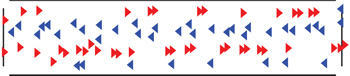
In the theater, subway station, airport or other public places, there always exist corridors having bidirectional flows. It is a very meaningful job to understand flow efficiency that may be affected by different types of flows in order to avoid breakdown to occur as much as possible. This paper assumes that the bidirectional pedestrian flow moves in a corridor whose size is 10 m × 4 m as shown in Fig. 1. The inflows of pedestrians on both sides are from the outside of the corridor which are considered to be controllable, and we set the initial speeds for pedestrians are 0.5 m/s in this paper. Besides, the distance between the place where pedestrians come from and the entrance of the corridor is 1 m in order that pedestrians can achieve the normal walking states in the corridor. Once pedestrians leave the corridor (10 m × 4 m), they can still keep walking forward according to the social force model until totally passing the place where the inflows come from. Assume that the inflow from each side of the corridor maintains a constant value in each simulation, and the ratio between the inflows from both sides is one to one.
Fig. 1. The snapshot of the simulated bidirectional pedestrian flow.
In order to study the dynamic features in the homogeneous and heterogeneous bidirectional flows, Table 2 presents 16 scenarios by changing the parameters in the social force model, namely, desired velocity, reaction time, and body size. The reasons why we consider them as variables are a decrease in free speed, diminishing maneuverability, and an increase in individual size.[18] It should be noted that scenario 0 is set as the reference scenario. Only one parameter in scenarios 1–15 replaces the corresponding parameter in the reference scenario, and others remain the same. We assume that pedestrians’ reaction time τ uniformly distributes between 0.20 s and 0.50 s with its deviation στ in scenarios 6 and 7, and radius r uniformly distributes between 0.200 m and 0.300 m with its deviation σr in scenarios 11 and 12. Pedestrians’ desired velocity, however, satisfies the normal distribution with the standard deviation σv in scenarios 1 and 2. Scenario 5 refers to pedestrians on both sides either having faster desired speeds 1.50 m/s or slower desired speeds 1.20 m/s, and the number of pedestrians with faster desired speeds is the same with that with slower ones. Analogously, we set the scenarios 10 and 15.
Table 2.
Table 2.
Table 2.
Parameter settings in different simulation scenarios.
.
Simulation scenarioa
Reaction time τ/s
Deviation στ
Desired Speed v0/(m/s)
Standard deviation σv
Radius r/m
Deviation σr
0: The reference scenario
0.35
0.00
1.35
0.0
0.250
0.000
1: Medium heterogeneity in desired speed
0.2
2: Large heterogeneity in desired speed
0.4
3: Low desired speed
1.20
4: High desired speed
1.50
5: Two different desired speeds
1.20/1.50
6: Medium heterogeneity in reaction time
0.05
7: Large heterogeneity in reaction time
0.10
8: Short reaction time
0.20
9: Long reaction time
0.50
10: Two different reaction time
0.20/0.50
11: Medium heterogeneity in body size
0.025
12: Large heterogeneity in body size
0.050
13: Small body size
0.200
14: Large body size
0.300
15: Two different body sizes
0.200/0.300
Table 2.
Parameter settings in different simulation scenarios.
.
The performance of free flows is characterized by the mean speed of the flow and the fluctuation in speed. The performance of congestion flows, however, is indicated by the breakdown probability and the start time of breakdown.
4. Analysis of the free flow
In the free bidirectional flow, pedestrians can walk freely and lanes start to form. In this section, the detailed comparisons and interpretations of pedestrians’ movement in different scenarios of Table 2 are presented in order to analyze the behaviors of the bidirectional pedestrian flow.
4.1. Free speed analysis of flows with differences in desired speed
The walking speed and flow rate are two important parameters to reflect the free flow dynamics to some degree. Generally, the flow rate is not only related to the walking speed but also to the density of pedestrians. After the repeated simulation runs, we find that the flow rates in different scenarios of Table 2 are close to each other. Take scenarios 0–5 for example, the flow rates and the corresponding standard deviations are presented in Table 3. It can be observed that the mean values of flow rates obtained from 20 simulation runs respectively are similar to each other. The standard deviations in Table 3, however, can still reflect some phenomena, such as the largest value of standard deviation in scenario 2 showing that the large heterogeneity in desired speed has relatively large effects on the free pedestrian flow. In this paper, only the walking speed in the free flow is used to analyze pedestrians’ behaviors in the bidirectional flow. By analyzing the free walking speed, we can not only obtain the detailed walking behaviors of the free flows reflected from the simulation results of the flow rates but also find some new movement characteristics in different scenarios.
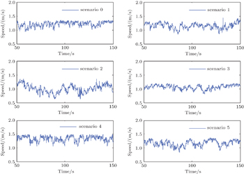
Figure 2 shows the time evolution of speeds during a simulation for bidirectional flows in scenarios 0–5. Actually, the speed at each time instant in Fig. 2 is the mean value of all pedestrians’ speeds, and pedestrians update their own speeds according to the social force model after each time step ΔT. ΔT is set to 0.1 s during the simulation which considers many factors such as avoiding overlapping. Note that we choose the time period from 50 s to 150 s to eliminate the effect of initial conditions, and the inflow is set to 1 p/s from both sides. Table 4 respectively presents the mean value and standard deviation of speed for scenarios 0–5 after 20 simulation runs and also presents the corresponding results for the simulation in Fig. 2. From the mean speeds and standard deviations obtained after one simulation run, we can observe that these values are basically close to the corresponding values obtained after 20 simulation runs. Therefore, the simulation results shown in Fig. 2 are not from the special cases, and these results can reflect the evolution of speed over time for different scenarios 0–5.
Fig. 2. Time evolution of flow speeds for scenarios 0–5.
Table 4.
Table 4.
Table 4.
Analysis of the free speeds for scenarios 0–5.
.
Scenario 0
Scenario 1
Scenario 2
Scenario 3
Scenario 4
Scenario 5
Mean speed/(m/s) (20 simulation runs)
1.19
1.14
0.94
1.04
1.34
1.17
Standard deviation (20 simulation runs)
0.09
0.11
0.15
0.10
0.10
0.10
Mean speed/(m/s) (1 simulation run)
1.20
1.14
1.00
1.06
1.34
1.17
Standard deviation (1 simulation run)
0.09
0.10
0.15
0.08
0.10
0.1
Table 4.
Analysis of the free speeds for scenarios 0–5.
.
It can be clearly observed that there is a positive correlation between the value of desired speed less than a critical threshold and the mean speed by comparing the data of scenarios 0, 3, and 4 in Table 4. Furthermore, we can find that the speed of the bidirectional flow in scenario 2 fluctuates greatly with the largest standard deviation 0.15, and the mean speed in scenario 2 is also the smallest among these six scenarios by comparing the curves in Fig. 2 and data in Table 4. It can be drawn that the large heterogeneity in desired speed has a very significant influence on the free flows. It can be comprehended that pedestrians with very slow desired speeds cannot even reach the average desired speed and overtaking behaviors occur which can result in small jam clusters. However, these small clusters, which may result in the instantaneous instability in speed, can be broken up when pedestrians in the clusters pass through each other after a few moment. It is worth noting that the mean desired speeds in scenarios 0 and 5 are the same which are both 1.35 m/s, and their mean speeds and standard deviations are also similar to each other. The temporary large fluctuations in speed in scenario 5 can be prevented even though the difference in desired speed is large. Therefore, the question is whether overtaking behavior in scenario 5 only has little influence on the movement of flow?
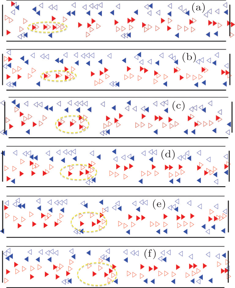
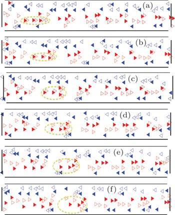
Fig. 3. Snapshots of walking states at different time instants: (a) t = 140 s, (b) t = 142 s, (c) t = 144 s, (d) t = 146 s, (e) t = 148 s, (f) t = 150 s.
In order to have a deeper understanding of the effect of the difference of desired speeds in scenario 5, we set the following symbols which can help to better analyze the motion features of the bidirectional flow: in Fig. 3, the solid triangles represent pedestrians with faster desired velocities, while hollow triangles represent pedestrians with slower desired velocities. Pedestrians with the red mark walk from left to right and pedestrians with the blue mark walk from right to left, which can also be distinguished from the pointing direction of triangles. Note that some unique moving states in scenario 5 may be missed or not very obvious to be found because the length of the corridor is too short or the difference between the high desired speed and low desired speed is too small. We, therefore, extend the corridor to 50 m, and set the faster desired speed and slower desired velocities vmin0 = 1 m/s to enlarge the differences between pedestrians. The width of the corridor remains the same which is 4 m and the inflow is set to 1 p/s.
From the movement of pedestrians within the yellow oval in Fig. 3, we can see people with faster desired speeds walk behind the pedestrians with slower desired speeds when t = 140 s, but overtaking behavior occurs after a few seconds. In a lane, there always exist pedestrians with faster desired speeds and also with slower ones, but we can find an interesting phenomenon that pedestrians with the same desired velocities tend to follow each other to develop a queue in a small scale. This lane formation is inside a lane. It can be explained as: Assume a moving state that there is no local lane formation inside a typical lane of the bidirectional flow, then pedestrians with faster desired speeds or with slower ones may walk together in a queue, and have the same desired walking direction to leave the corridor. According to Eqs. (1) and (2), pedestrians with faster desired speeds obtain larger desired forces which may result in the overtaking behavior or jam-cluster occurring, and the current moving state will be broken. Therefore, this temporary moving state above is not stable. On the contrary, if there exists the local lane formation inside a typical lane, a queue will contain pedestrians with the same desired speed in a small scale. These pedestrians bear the total driven force with the small differences coming from fi j which can result in the current moving state to remain stable for a while to realize the local equilibrium. The local inner lanes usually form after a series of unstable moving states. Note that the lanes are always broken and re-formed after a period of time especially on the boundaries because of the entrance of new pedestrians.
4.2. Free speed analysis of flows with differences in reaction time
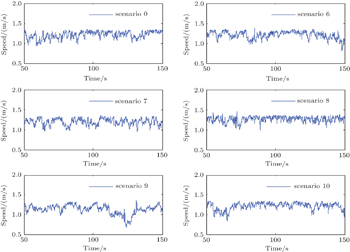
Figure 4 exhibits the time evolution of speeds during a simulation for scenarios 6–10. Table 5 respectively presents the mean value and standard deviation of speed for scenarios 6–10 after 20 simulation runs and also presents the corresponding results for the simulation in Fig. 4. The reason why listing the mean speed and standard deviation of one simulation run in Table 5 is the same with that in Table 4. When analyzing Fig. 4 and Table 5, it is easy to observe that not only the speed in scenario 9 is relatively slow, but also the standard deviation of mean speeds is relatively large. We can understand as pedestrians with long reaction time need more time to accelerate to the desired velocities, which may result in small jam clusters. Besides, the free speeds and the standard deviations in scenarios 6, 7, and 10 are similar to those in scenario 0. This reflects that the heterogeneity in reaction time does not play an important role in the free bidirectional pedestrian flows, and there is no need to deliberately distinguish pedestrians who are with different values of reaction time in scenarios 6 and 10.
Fig. 4. Time evolution of flow speeds for scenarios 6–10.
Table 5.
Table 5.
Table 5.
Analysis of the free speeds for scenarios 6–10.
.
Scenario 6
Scenario 7
Scenario 8
Scenario 9
Scenario 10
Mean speed/(m/s) (20 simulation runs)
1.20
1.20
1.26
1.08
1.20
Standard deviation (20 simulation runs)
0.09
0.09
0.07
0.16
0.08
Mean speed/(m/s) (1 simulation run)
1.21
1.19
1.26
1.13
1.21
Standard deviation (1 simulation run)
0.09
0.08
0.07
0.12
0.09
Table 5.
Analysis of the free speeds for scenarios 6–10.
.
4.3. Free speed analysis of flows with differences in body size
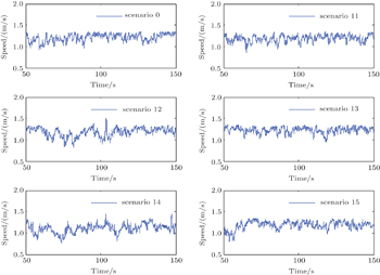
Figure 5 shows the time evolution of speed for scenarios 11–15, and Table 6 respectively presents the mean value and standard deviation of speed for scenarios 11–15 after 20 simulation runs and also presents the corresponding results for the simulation in Fig. 5. The reason why listing the mean speed and standard deviation of one simulation run in Table 6 is the same with that in Table 4. we can observe that the heterogeneity in body size does not have any important effect on the free moving state of the bidirectional flow by comparing the simulation results of scenarios 0, 11, and 12. Analogously, the free speeds in scenario 15 and scenario 11 are also close to each other. Moreover, the flow efficiency can be slightly improved if this flow contains homogeneous pedestrians with small body size. It is worth noting that the speed of homogeneous bidirectional flows with large body size has a smaller value and more fluctuations. It can be comprehended that the number of pedestrians walking in the corridor is limited because of the layout of the corridor and non-overlapping of pedestrians. The inflow, however, is determined and cannot change. Therefore, clusters or even breakdown may emerge at this time which can result in fluctuations in speed.
Fig. 5. Time evolution of flow speeds for scenarios 11–15.
Table 6.
Table 6.
Table 6.
Analysis of the free speeds for scenarios 11–15.
.
Scenario 11
Scenario 12
Scenario 13
Scenario 14
Scenario 15
Mean speed/(m/s) (20 simulation runs)
1.19
1.20
1.23
1.18
1.20
Standard deviation (20 simulation runs)
0.09
0.09
0.08
0.15
0.09
Mean speed/(m/s) (1 simulation run)
1.19
1.18
1.22
1.11
1.19
Standard deviation (1 simulation run)
0.08
0.11
0.07
0.11
0.10
Table 6.
Analysis of the free speeds for scenarios 11–15.
.
5. Breakdown phenomenon study
The moving bidirectional flow could transit from free flow to congestion flow under some circumstances, and breakdown may occur after congestion starts. Literature showed that different pedestrians have different features such as habits and physical states, and these different features may result in breakdown. In this section, we will focus on the breakdown issue of the bidirectional flow for the scenarios in Table 2. By comparing the simulation results, we can obtain which factor in pedestrians can result in breakdown more easily. In particular, the start time of breakdown is discussed in details, focusing on the range and the mean value of this start time.
Corresponding to Ref. [18] where the size of the corridor is the same with the one in our paper, total breakdown is defined when at least 60 pedestrians walk very slowly during five consecutive seconds. Here, we assume that this slow velocity has a maximum value of 0.2 m/s.
During our simulation the inflow value is constant even though the breakdown occurs, and each simulation lasts 1500 s. The statistics results, namely the breakdown probability and the start time of breakdown, are obtained after 100 simulation runs. It should be noted that 1500 s for each simulation is long enough for the study of breakdown because the length of the corridor is 10 m, and a pedestrian only needs about 10 s to pass the corridor in the free flow.
5.1. Analysis of breakdown probability
Figure 6(a) reflects the trend that breakdown probability rises when increasing inflow until it approaches 1 as expected. By analyzing this figure, we can find that the values of the homogeneous reaction time and body size in the social force model play more important roles in affecting the breakdown probabilities than the heterogeneities in these two parameters. Besides, the large heterogeneity in desired speed has a significant effect on breakdown probability, this may be because overtaking behaviors occur frequently which can result in disorders, congestion or even breakdown.
Fig. 6. The breakdown probability versus inflow of pedestrians. (a) Breakdown probabilities for scenarios 0–15, (b) breakdown probabilities classified by desired velocity, (c) breakdown probabilities classified by reaction time, (d) breakdown probabilities classified by body size.
Figure 6(b) shows the breakdown probability varying with inflow for different scenarios classified by the desired speed. What is clear is that both large heterogeneity in desired speed and low desired velocity less than a critical threshold result in breakdown to occur with larger probabilities under the same inflow. Besides, the relatively high desired speed less than a critical threshold can reduce breakdown to occur under a certain inflow from the simulation results. This critical value is 1.5 m/s according to Ref. [13]. Helbing et al. pointed that if the desired speed of pedestrians is lower than 1.5 m/s, the efficiency of leaving will increase with an increase in desired speed; and if the desired speed is higher than 1.5 m/s, the efficiency of leaving will decrease with increasing the desired speed because of pushing which can result in additional friction effects.[13] Accordingly, it is not the arbitrarily large desired speed can reduce the breakdown probability. We can further conclude that if smaller breakdown probability is expected to be obtained in the bidirectional flow, this pedestrian flow should better contain more pedestrians with relatively high desired speed less than the threshold value, and pedestrians’ desired speeds should better have smaller heterogeneities.
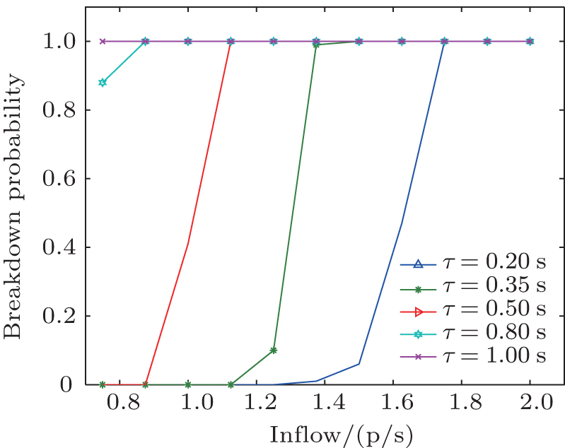
Figure 6(c) shows the relationship between the breakdown probability and the inflow for different scenarios classified by reaction time. From this figure, we can find that scenarios 0, 6, 7, and 10 have similar breakdown probabilities under the same inflow, for example we choose inflow to be 1.25 p/s, the breakdown probabilities are respectively 0.1, 0.09, 0.04, 0.06 which exist very small differences. This implies that the heterogeneity in reaction time does hardly affect the breakdown probability under a certain inflow. The size of reaction time, however, plays an important role. In a certain range of reaction time, the longer the reaction time is, the larger the breakdown probability of the bidirectional flow becomes as figure 7 shows. This relationship between reaction time and breakdown probability does not change when reaction time becomes longer. The reason is that pedestrians with the homogeneous shorter reaction time can adjust their desired velocity quickly according to the realtime surroundings, while pedestrians with the homogeneous longer reaction time usually have lags in response which can reduce the flow efficiency. Note that in Fig. 7 pedestrians in the bidirectional flow have the homogeneous reaction time with different values, and other parameters remain the same in all simulation runs.
Fig. 7. The breakdown probability versus inflow for scenarios with the homogeneous reaction time.
Figure 6(d) presents the breakdown probability versus inflow for different scenarios classified by body size. The heterogeneity in body size does not play any major role in breakdown probability, even though it has more impacts than the heterogeneity in reaction time. The value of homogeneous body size, however, can affect the breakdown probabilities significantly. The trend that the breakdown probability increases with an increase in body size does not change, and the reason for this is similar to that presented in the end of section 4.3.
5.2. Analysis of the start time of breakdown
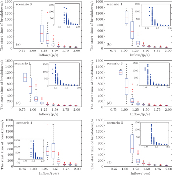
The start time of breakdown with the change of inflow for the scenarios in Table 2 are studied and analyzed to have a more in-depth understanding of breakdown. Figures 8(a)–10(e) show the box-plots for the scenarios in this paper. In each box-plot, the central red mark represents the mean value of the start time of breakdown under each inflow, and the bottom and top edges of the blue box represent the 25th and 75th percentiles of all collected data. Besides, the dashed lines respectively extend to the maximum and minimum values not considering outliers, and red outliers are plotted separately.
Fig. 8. The start time of breakdown versus inflows classified by desired speed. (a) Box-plot for the reference scenario, (b) box-plot for pedestrians with medium heterogeneity in desired speed, (c) box-plot for pedestrians with large heterogeneity in desired speed, (d) box-plot for pedestrians with homogeneous low desired speed, (e) box-plot for pedestrians with homogeneous high desired speed, (f) box-plot for pedestrians with two different desired speeds.
Figures 8(a), 8(b), and 8(c) respectively present the box-plots of the start time of breakdown for pedestrians with no, medium and large heterogeneities in desired speed. Note that the subgraph in each figure shows the collected simulation data of the start time of breakdown. By comparing the mean value of boxes under the same inflow, we can observe that large heterogeneity in desired speed has the largest impact on the start time of breakdown which can result in breakdown to start early. The medium heterogeneity in desired speed also has influence on the start time of breakdown, but not as much as the large heterogeneity does.
By comparing Figs. 8(a), 8(d), and 8(e), it is very clear that desired speed is very important to the movement state of the bidirectional flow. The homogeneous high desired speed less than a critical threshold can result in breakdown to occur late or even not take place under low inflows. By observing Figs. 6(b), 8(a), and 8(f), we can find that the probability of breakdown in the scenario 5 which contains pedestrians with two different desired speeds is only a little higher than that in the reference scenario, and the mean value of the start time of breakdown in scenario 5 is similar to that in the reference scenario. The reason for this is explained in the previous section.
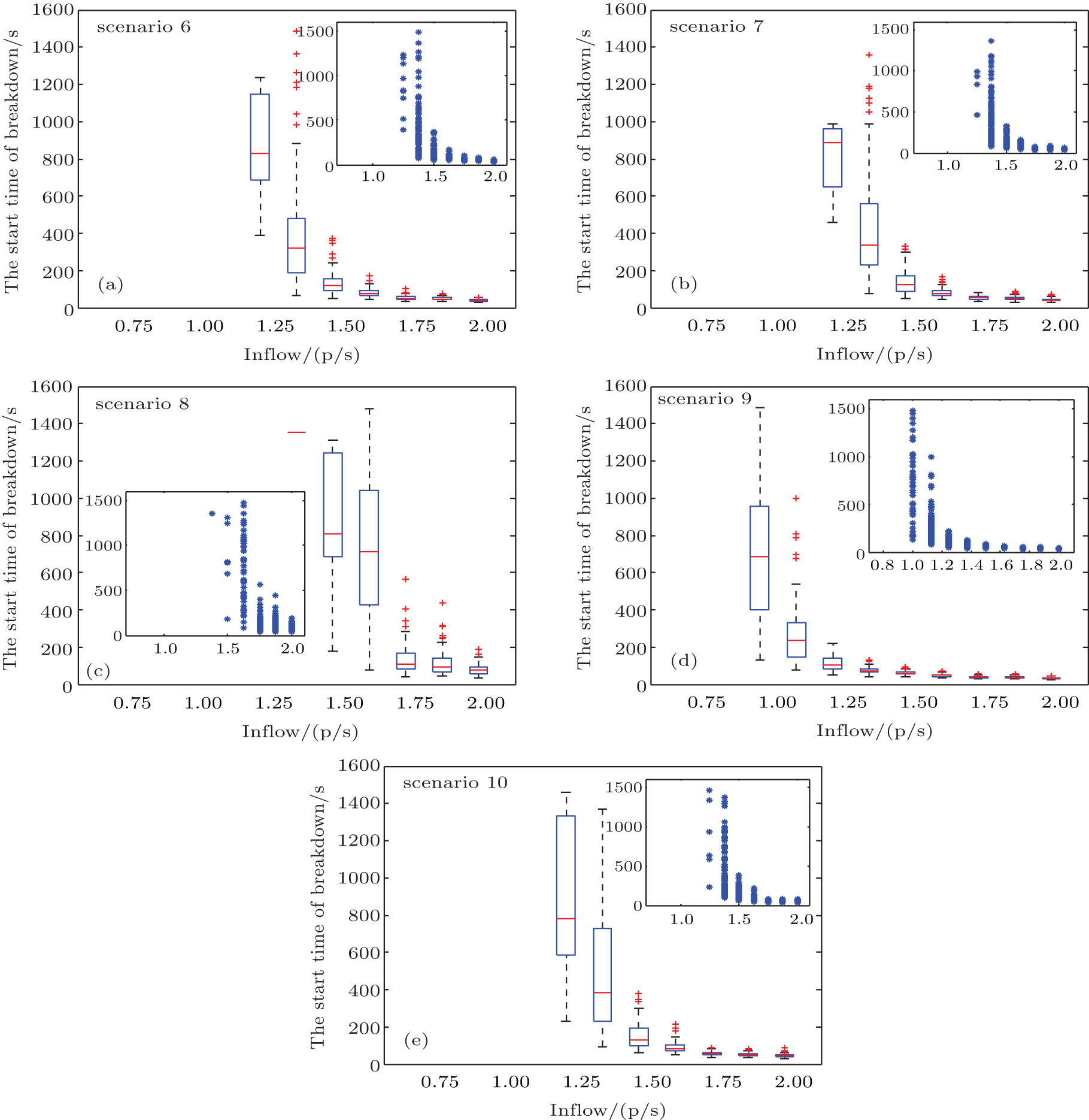
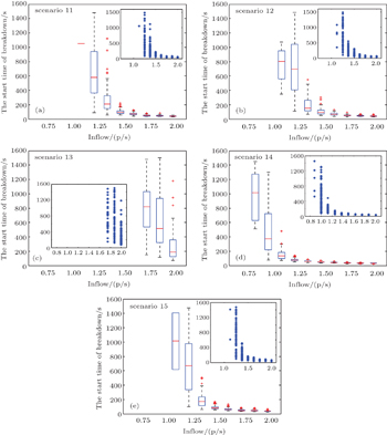
Comparing Figs. 8(a), 9(a), and 9(b), we can see that the heterogeneity in reaction time does not have an important effect on the start time of breakdown. The reaction time value, however, plays an important role on the start time of breakdown which can be clearly seen in Figs. 9(c) and 9(d). Figure 9(e) shows that there is not any large difference in the start time of breakdown between scenario 10 and the reference scenario. Therefore, there is no necessary to consider the effect of heterogeneity in reaction time on the start time of breakdown.
Fig. 9. The start time of breakdown versus inflows classified by reaction time. (a) Box-plot for pedestrians with medium heterogeneity in reaction time, (b) box-plot for pedestrians with large heterogeneity in reaction time, (c) box-plot for pedestrians with homogeneous short reaction time, (d) box-plot for pedestrians with homogeneous long reaction time, (e) box-plot for pedestrians with two different reaction time.
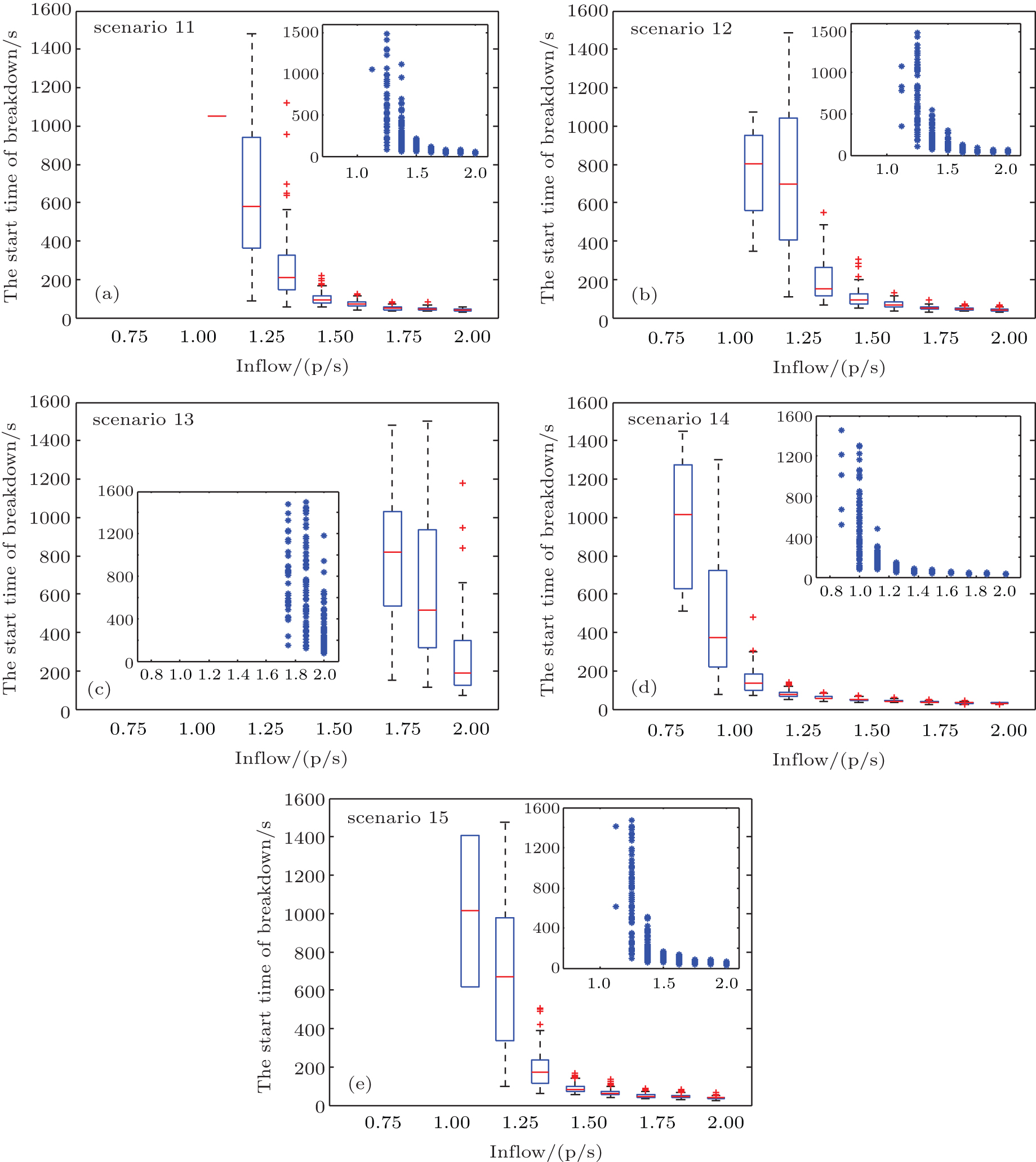
Through comparing Figs. 10(a)–10(d), we can conclude that the size of body size is closely related to the start time of breakdown. As is expected, the homogeneous small body size can not only decrease the probability of breakdown but also result in breakdown to start late. Besides, the effect of the heterogeneity in body size on the start time of breakdown is not so much compared with the effect of the size of body size. By comparing Figs. 10(e), 8(a) and 6(d), we can obtain that both the breakdown probability and the start time of breakdown in scenario 15 which contains the pedestrians with two different body sizes are similar to those in the reference scenario.
Fig. 10. The start time of breakdown versus inflows classified by body size. (a) Box-plot for pedestrians with medium heterogeneity in body size, (b) box-plot for pedestrians with large heterogeneity in body size, (c) box-plot for pedestrians with homogeneous small body size, (d) box-plot for pedestrians with homogeneous large body size, (e) box-plot for pedestrians with two different body sizes.
By analyzing Figs. 8(a)–10(e), it is very distinct that the mean value of the start time of breakdown decreases with increasing inflow in each scenario. Therefore, an increase in inflow not only results in a higher breakdown probability of occurring as expected, but also results in breakdown to start early. Generally speaking, the smaller the value of the start time of breakdown under the same inflow for the scenarios in Table 2, the larger the effect of the corresponding factor on breakdown. For example, we take a look at Figs. 8(b) and 8(c). Under the inflow 1.25 p/s, the mean start time of breakdown in scenario 2 is smaller than that in scenario 1, this reflects that the large heterogeneity in desired velocity has a larger effect on breakdown than the medium heterogeneity does which can also be obtained from Fig. 6. By the comprehensive analysis of Fig. 6 and Figs. 8–10, we can find the relevancy between breakdown probabilities and the start time of breakdown. Basically, under a certain inflow the smaller the start time of breakdown is, the larger the breakdown probability becomes which can be drawn from Table 7, thereby the larger effects on breakdown. However, there do exist exceptions. For example, under the inflow is 1.25 p/s, both the start time of breakdown and the breakdown probability in scenario 0 are smaller than those in scenario 1. This may be because the collected simulation data of the start time of breakdown are not enough. Generally, the number of the collected data of the start time of breakdown is related not only to the number of simulation runs which is 100 in this paper but also to the corresponding breakdown probability. Therefore, we can only obtain 10 simulation data of the start time of breakdown in scenario 0 when inflow is 1.25 p/s. Breakdown does not occur sometimes during the repeatable simulations for low inflows, this is the reason why the subgraph has less points for low inflows. Moreover, we can observe that the start time of breakdown will be relatively concentrated and vary slightly if inflow is relatively high, when it is easier to predict the start time of breakdown.
Table 7.
Table 7.
Table 7.
The comparison of simulation results of breakdown for scenarios 0–2.
.
Table 7.
The comparison of simulation results of breakdown for scenarios 0–2.
.
In sum, from the simulation results it can be drawn that the sizes of the three parameters in the social force model, namely, the desired speed, reaction time, and body size, not only play an important role in breakdown probability of the bidirectional flow but also have a significant influence on the start time of breakdown. The heterogeneity in desired speed has a much larger impact on breakdown than that in reaction time or in body size does, and the effect of the heterogeneity in body size on breakdown is a little larger than that in reaction time.
6. Conclusion
Based on the social force model, we have presented and analyzed the dynamic features of the bidirectional pedestrian flow for sixteen different scenarios in this paper. The speeds in the free flows are focused on for the homogeneous and heterogeneous studies of the effects of the parameters in the social force model on the flow dynamics. The simulation results show that the homogeneous higher desired speed less than a critical threshold, shorter reaction time or smaller body size can yield higher free speed of the bidirectional flow. In particular, the large heterogeneity in desired speed results in the free speed to become slow and together with frequent fluctuations in the instant, while the heterogeneity in reaction time or in body size does not play an important role in free flows. Moreover, the breakdown probability and the start time of breakdown for different scenarios are considered and analyzed. We can draw our conclusion that heterogeneity in desired speed which can not only result in breakdown probability to become larger but also affect breakdown to occur earlier has larger impacts on breakdown than that in reaction time or body size. Besides, the homogeneous higher desired speed less than a critical threshold, short reaction time or small body size can delay the start time of breakdown.
Our study provides the effect of different types of pedestrian flows on the flow efficiency, which can not only enlighten us to understand more about the dynamics of bidirectional flows but also provide some theoretical supports to assess the layout of corridor in the facility design under the expected traffic to avoid jams or even breakdown. Moreover, the best design of the corridor can be implemented with a pre-determined probability of breakdown for different types of pedestrians. Our future work will in particular focus on the lane formation of the bidirectional flow such as the time evolution of the number of lanes and the width of lanes.


 , Yao Xiu-Ming3]