Numerical investigation of a coupled moving boundary model of radial flow in low-permeable stress-sensitive reservoir with threshold pressure gradient
Liu Wen-Chao, Liu Yue-Wu†, , Niu Cong-Cong, Han Guo-Feng, Wan Yi-Zhao
Institute of Mechanics, Chinese Academy of Sciences, Beijing 100190, China


† Corresponding author. E-mail: liuyuewulxs@126.com

Project supported by the National Natural Science Foundation of China (Grant No. 51404232), the China Postdoctoral Science Foundation (Grant No. 2014M561074), and the National Science and Technology Major Project, China (Grant No. 2011ZX05038003).

Abstract
Abstract

The threshold pressure gradient and formation stress-sensitive effect as the two prominent physical phenomena in the development of a low-permeable reservoir are both considered here for building a new coupled moving boundary model of radial flow in porous medium. Moreover, the wellbore storage and skin effect are both incorporated into the inner boundary conditions in the model. It is known that the new coupled moving boundary model has strong nonlinearity. A coordinate transformation based fully implicit finite difference method is adopted to obtain its numerical solutions. The involved coordinate transformation can equivalently transform the dynamic flow region for the moving boundary model into a fixed region as a unit circle, which is very convenient for the model computation by the finite difference method on fixed spatial grids. By comparing the numerical solution obtained from other different numerical method in the existing literature, its validity can be verified. Eventually, the effects of permeability modulus, threshold pressure gradient, wellbore storage coefficient, and skin factor on the transient wellbore pressure, the derivative, and the formation pressure distribution are analyzed respectively.

1. Introduction

In modern times, these unconventional tight oil and gas reservoirs such as oil & gas shale reservoirs and low-permeable reservoirs have become new energy targets in petroleum engineering; and they play more and more important roles in the world’s energy consumption. Correspondingly, the studies of the kinematic principles of fluid flow in unconventional reservoirs and their applications in engineering problems have become a hot topic at present.

1.1. Moving boundary problem considering threshold pressure gradient

Abundant experimental and theoretical analyses[113] have demonstrated that the fluid flow in low-permeable reservoirs do not obey the conventional Darcy’s law; there exists a threshold pressure gradient (TPG). That is, the fluid flow happens only if the formation pressure gradient exceeds TPG. In particular, Cai[11] presented the analytical expressions for the flow rate and the velocity of non-Newtonian fluid flow in low-permeable porous medium, and also obtained the scaling relation between TPG and permeability through fractal approach.

Unlike the modeling of Darcy’s flow, the flow in porous medium with TPG is a nonlinear moving boundary problem. Figure 1 shows the computed dimensionless formation pressure distribution curves corresponding to Darcy’s flow and the flow in porous medium with TPG, respectively. Compared with the result of Darcy’s flow, the dimensionless formation pressure distribution curve of modified Darcy’s flow is much steeper, and the dimensionless formation pressure becomes zero value at the position of moving boundary. At the moving boundary, the formation pressure gradient is just equal to TPG. Inside the moving boundary, the dimensionless formation pressure gradient is larger than TPG, and then the fluid flow can be driven under a net pressure gradient, i.e., the formation pressure gradient minus TPG. However, outside the moving boundary, no fluid flow happens (the formation pressure keeps initial pressure; and the formation pressure gradient is equal to zero, which is a “jump” of pressure gradient at the moving boundary position). In a word, the formation pressure curve corresponding to modified Darcy’s flow shows a property of compact support.[10]

Fig. 1. Comparison between computed dimensionless formation pressure distribution curves with and without including TPG.

In another way, if an angle α between formation pressure curve and distance is set to be on the moving boundary, TPG will be equal to the value of tangent α from the definition of TPG. When TPG tends to zero, the tangent of α will become zero gradually. Then the type of formation distribution curve will tend to a limit case i.e., Darcy’s flow.

Many relevant studies have proved that it is very significant to take into account the TPG in the modeling of fluid flow in porous medium in low-permeable reservoir, whether from reservoir engineering applications or theoretical modeling analysis. For example, the gas flow in water bearing tight gas reservoirs in consideration of TPG is investigated by Zhu et al.;[14] and through the analytical investigation, their presented mathematical model shows that due to the existence of TPG the reservoir energy is largely consumed near the wellbore. The research[15] by Zhu et al. shows that the considering of TPG in low-permeable reservoir simulation can improve the history matching precision in the relevant applications in Units X10 and X11 of Daqing Oilfield. In Yin and Pu’s study,[16] it is demonstrated through a pilot test in Chao 45 Block of Daqing Oilfield that the improved history matching degree can be reached under the condition of considering TPG in the simulation of surfactant flooding in low-permeable reservoir. Yao et al.[10] and Liu et al.[17] investigated a basic one-dimensional moving boundary problem of fluid flow in porous medium with TPG by an analytical solution method and a subsequent strictly verified numerical method. And it is concluded that it is very necessary to take into account the effect of TPG for the fluid flow in porous medium with TPG, for mathematical modeling in engineering applications.

1.2. Stress-sensitive effect

In the actual oil and gas production, the fluid pressure in the development of oil and gas from low-permeable reservoirs decreases gradually with the production time. As a result, the rock skeleton, which bears the net overburden pressure of reservoirs, will be compressed and deformed. It can cause elastoplastic deformation of the rocks, and reduce the permeability of reservoir. Academically, it is defined as “stress-sensitive reservoir”.[1823] However, as far as we know, in previous researches of the moving boundary problems of fluid flow in low-permeable reservoir, the effect of deformation of low-permeable rock has not been considered and evaluated yet.

Here, based on these aforementioned concerns, in consideration of the two prominent physical phenomena in the development of low-permeable reservoirs i.e., the existence of TPG and the stress-sensitive effect, a new coupled moving boundary model of radial flow in low-permeable reservoir is developed; a concept of permeability modulus[18,19,21,22] is introduced to reflect the effect of formation deformation on the permeability change. Besides, both the wellbore storage and skin effect are incorporated into the inner boundary conditions.

Abundant researches have been conducted on the analytical and numerical solutions for such moving boundary problems of fluid flow in porous medium with TPG. And current major solution methods include the integral approximate analytical method,[24] the Green function method,[25] the exact analytical solution by similarity transformation method,[17,26] coordinate transformation based numerical method,[10] and direct finite difference numerical method.[27] Owing to the strong nonlinearity and complexity of our presented coupled moving boundary model, a coordinate transformation based finite difference method[10] is adopted to numerically investigate the effect of physical parameters on the model solutions to the formation pressure and moving boundary. The utility of the numerical method can be attributed to its simple approach to converting the moving boundary problem into a problem with fixed boundary conditions, and then solving it by a stable fully implicit finite difference method on fixed spatial grids.

2. Mathematical modeling
2.1. Physical model

The problem considered involves the radial flow in an infinite low-permeable stress-sensitive reservoir with TPG. The reservoir is homogeneous, isotropic, and isothermal. And the single-phase horizontal flow does not have any gravity effect. Both the wellbore storage and skin effect[19] are considered. The Newtonian fluid and rocks are slightly compressible.

The schematic of the physical model is shown in Fig. 2. Once the oil is produced from the low-permeable reservoir with TPG, the formation pressure drop happens in the formation inside the moving boundary. Owing to the formation pressure drop, the stress −sensitive reservoir can be deformed, which reduces the formation permeability (See Fig. 2).

Fig. 2. Schematic diagram of physical model.
2.2. Mathematical model

The fluid density is as follows:[24]

where ρ is the fluid density (in units g·cm− 3); ρ0 is the initial fluid density (in units g·cm− 3); p0 is the initial pressure (in unit atm); p is the pressure (in unit atm, 1 atm = 1.01325×10⁵ Pa); Cf is the compression coefficient of the fluid (in unit atm− 1).

The porosity of the porous medium is as follows:[24]

where ϕ is the porosity of the porous medium (in the fraction form); ϕ0 is the initial porosity (in the fraction form); Cϕ is the compression coefficient of the porosity (in unit atm− 1).

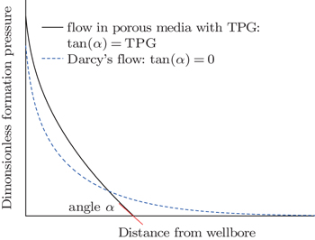
The modified Darcy’s law for the fluid flow in the porous medium with TPG is as follows:[1]

where k is the permeability of the porous medium (in unit D); μ is the fluid viscosity (in unit cP); r is the radial distance (in unit cm); υ is the seepage velocity (in units cm3·(s·cm2)− 1); λ is the TPG (in unis atm·cm− 1).

The permeability modulus γ (in unit atm− 1) is similar to the compressibility coefficient, and can be defined by the following equation:[18,19,21,22]

Coefficient γ plays an important role in the stress-sensitive effect on the rock permeability. It is a measurement of the dependence of the permeability on formation pressure drop. For practical engineering applications, it can be assumed to be constant.[18,19,21,22] Then the permeability of deformed rock in low-permeable reservoirs can be expressed from Eq. (4) as follows:

where k0 is the permeability at the initial reservoir pressure.

The continuous equation for the radial flow in the porous medium is as follows:[24]

where t is the time (in unit s); 
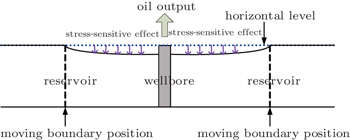
s is the moving boundary (in unit cm); rw is the wellbore radius (in unit cm). Besides, it should be noted that Eq. (6) is only valid for the radial space from the wellbore to the moving boundary.

Substituting Eqs. (1)–(3), and (5) into Eq. (6), the governing (mass balance) equation for the radial flow in the low-permeable stress-sensitive reservoir, can be deduced as follows:

where Ct is the total compression coefficient (in unit atm− 1); and Cfγ.

The initial conditions are as follows:

The inner boundary conditions in consideration of wellbore storage and skin effect with constant flow rate are

where h is the reservoir thickness (in unit cm); C is the coefficient of wellbore storage (in units cm3·atm− 1); q is the constant flow rate (in units cm3·s− 1); B is the volume factor, dimensionless; pwf is the wellbore pressure (in unit atm); S is the skin factor.

According to the definition of TPG, the moving boundary conditions are the same as the ones in Ref. [10] as follows:

Equations (7)–(13) together form a coupled moving boundary model of radial flow in low-permeable stress-sensitive reservoir with TPG for the case of a constant flow rate at the inner boundary in consideration of both the wellbore storage and skin effect.

The dimensionless variables are defined as follows:

where 
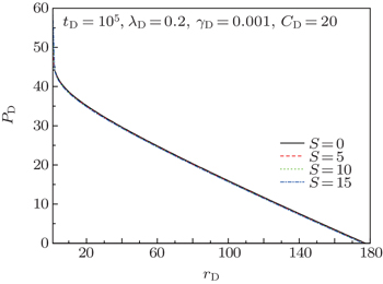
rD is the dimensionless radial distance; tD is the dimensionless time; PD is the dimensionless pressure; 
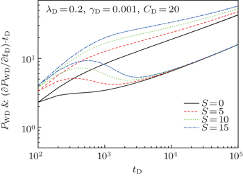
PwD is the dimensionless wellbore pressure; αD is the dimensionless compressibility; λD is the dimensionless TPG; γD is the dimensionless permeability modulus; 
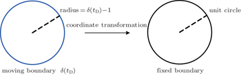
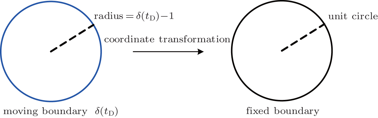
δ is the dimensionless moving boundary; CD is the dimensionless coefficient of wellbore storage.

And then the dimensionless form of the coupled moving boundary model can be transformed equivalently. The governing equation is as follows:

The initial conditions are as follows:

The inner boundary conditions are as follows:

The moving boundary conditions are

3. Velocity of moving boundary

From Eq. (28), we have

Differentiating two sides of Eq. (29) with respect to tD, we have

Substituting Eq. (27) into Eq. (30) yields

By using Eqs. (27) and (28) and letting xD = δ (tD) on both sides of Eq. (22), we have

By Eqs. (31) and (32), the velocity of the moving boundary can be written as follows:

.

From Eq. (33), it can be concluded that the velocity of moving boundary is proportional to the second derivative of the formation pressure function with respect to the radial distance on the moving boundary, but inversely proportional to TPG. It is different from the result of classical heat-conduction Stefan problem.[15,17]

4. Numerical method

In order to overcome the difficulty in discretizing space for the transient flow region with moving boundary, a spatial coordinate transformation method is used. It is the same as the one for the radial seepage flow problem with moving boundary in Ref. [10] as follows:

Through Eq. (34), the dynamic flow region for the moving boundary problem [0, δ(tD)] can be transformed into a fixed region [0, 1] as shown in Fig. 3. Then the dimensionless pressure PD(rD, tD) can be transformed into a new variable η (y, tD). The same transformation of differential variables as the one in Ref. [10] can be obtained as

Fig. 3. Schematic diagram of coordinate transformation.

Expanding the term on the left-hand side of the governing equation i.e., Eq. (22), the resulting equation can be obtained as follows:

Substituting Eqs. (35)–(37) into Eq. (38) yields

Substituting Eqs. (35)–(37) into Eq. (23), Eqs. (25)–(28), and Eq. (33), respectively, we have

From Eq. (43), we have

Substituting Eqs. (45) and (46) into Eq. (39) to cancel the variables ∂ δ/∂ tD and δ yields

Substituting Eq. (46) into Eqs. (41) and (42) to cancel the variables δ yields

Equations (47)–(49), Eq. (40) and Eq. (44) together form a transformed mathematical model with fixed boundary conditions. The model shows strong nonlinearity, indirectly indicating the strong nonlinearity of the original, untransformed moving boundary problem. Here, a stable, fully implicit finite difference method[10] is used to obtain its numerical solutions of the nonlinear model. The difference equation for the model can be written as follows:

where N denotes the total number of spatial grid subintervals with the same length; Δy is the length of a grid subinterval, which is equal to 1/N; i denotes the index of the spatial grid from the well; j denotes the index of a time step; ΔtD denotes the time step size.

Equations (50)–(54) together form the closed difference equations at the (j + 1)-th time step, and also contain (N + 1) unknown variables. The Newton–Raphson iterative method[10] is used to numerically solve these nonlinear difference equations. Eventually, numerical solutions for the transformed nonlinear partial differential equation system with respect to η (y, tD) can be obtained.

The difference equation of Eq. (46) is

Substituting Eq. (55) into the difference equation of Eq. (34) yields

By Eq. (56), numerical solutions of η (y, tD) can be transformed into the ones of PD(rD, tD) in the numerical solution process.

5. Verification of numerical solutions

Li and Liu[27] have studied a moving boundary model of radial flow in porous medium with TPG without consideration of the stress-sensitive effect, nor wellbore storage nor skin effect. Its numerical solution is obtained by direct spatial discretization with fixed grids. In our presented coupled moving boundary model, if γD, CD, and S are all set to be zero, the coupled moving boundary model can be reduced to the same model as the one in Ref. [27]. From Eq. (55), the dimensionless moving boundary distance δ can be computed for each time step. Then the numerical solutions regarding the dimensionless transient distance of moving boundary by the two different numerical methods can be compared with others.

Figure 4 shows the comparison between numerical results when the value of dimensionless TPG λD is equal to 0.0001. From Fig. 4, it can be seen that the two numerical solutions are in a good agreement. Therefore, the validity of the coordinate transformation based finite difference numerical method of solving the coupled moving boundary model presented here can be verified.

Fig. 4. Comparison of numerical results
6. Results and discussion
6.1. Effect of dimensionless permeability modulus γD

Figure 5 shows the effects of dimensionless permeability modulus on the log–log curves of dimensionless transient wellbore pressure and its derivative (with respect to dimensionless time) multiplied by the dimensionless time, under different values of dimensionless permeability modulus. These typical log–log curves are very useful for the well testing explanation in petroleum engineering. Figure 6 shows the effects of dimensionless permeability modulus on the dimensionless formation pressure distribution for different values of γD.

Fig. 5. Effects of dimensionless permeability modulus on transient wellbore pressure and its derivative for different values of γD.
Fig. 6. Effects of dimensionless permeability modulus on formation pressure distribution for different values of γD.

Figure 5 shows that the dimensionless permeability modulus, characterizing the reservoir deformation, has little effect on both the transient wellbore pressure and its derivative.

Figure 6 indicates that the larger the dimensionless radial distance, the bigger the effect of reservoir deformation on the formation pressure is; the larger the dimensionless permeability modulus, the nearer the dimensionless distance of moving boundary is. It can be explained that the reservoir deformation can reduce the formation permeability as the formation pressure drops, which slows down the propagation of moving boundary. Besides, it can be concluded from Fig. 6 that the larger the dimensionless permeability modulus, the bigger the sensitive effect of the parameter is.

With respect to the dimensionless formation pressure, near the wellbore (see the enlarged semi-log plot in the inset of Fig. 6), with the increase of the dimensionless radial distance, the larger the dimensionless permeability modulus, the larger the dimensionless formation pressure and the absolute value of the dimensionless formation pressure gradient are; however, in the place further away from the wellbore, with the increase of the dimensionless radial distance, the larger the dimensionless permeability modulus, the smaller the dimensionless formation pressure is. Then it can be concluded that the more serious pressure drop caused by the formation deformation in low-permeable reservoirs mainly happens in the place near the wellbore; it can be explained that much larger formation pressure drop happens near the wellbore than far away from the wellbore in the formation, and can cause greater formation deformation and subsequent permeability reduction.

6.2. Effect of dimensionless TPG λD

Figures 7 and 8 show the effects of dimensionless TPG λD on dimensionless transient wellbore pressure and its derivative, and dimensionless formation pressure distribution respectively, under different values of dimensionless TPG. The estimation of value range of λD has been performed from the experimental data of eight samples[1,10] and the range is from 0 to 0.852. Here four different values of λD are set to be 0.1, 0.2, 0.3, and 0.4, respectively.

Fig. 7. Effects of dimensionless TPG on transient wellbore pressure and its derivative.
Fig. 8. Effect of dimensionless TPG on formation pressure distribution.

From Figs. 7 and 8, it can be seen that the larger the dimensionless TPG, the larger the dimensionless transient wellbore pressure and its derivative are and the smaller the disturbed area between the wellbore and the position of moving boundary is. In comparison with the typical curves of Darcy’s flow, these log–log curves, which correspond to non-zero value of TPG, all turn upward, and the line representing the period of radial flow is not horizontal any more. The formation pressure distribution curve corresponding to larger TPG exhibits a larger slope. Moreover, unlike for Darcy’s flow problem, for this moving boundary problem, the formation pressure drops only inside the moving boundary, but outside the moving boundary the formation still keeps initial pressure: the pressure distribution curves show a property of compact support.[10]

Besides, from Fig. 7, it can also be concluded that the smaller the dimensionless TPG, the bigger the sensitive effects on the transient wellbore pressure and the derivative are, which challenges the well testing problems in low-permeable reservoirs.

6.3. Effect of dimensionless wellbore storage coefficient CD

Figures 9 and 10 show the effects of dimensionless wellbore storage CD on dimensionless transient wellbore pressure and derivative and dimensionless formation pressure distribution respectively, under different values of dimensionless wellbore storage coefficient CD.

Effects of dimensionless wellbore storage coefficient on transient wellbore pressure and its derivative for different values of CD.

Effects of dimensionless wellbore storage coefficient on formation pressure distribution for different values of CD.

From Fig. 9, it can be seen that the wellbore storage mainly affects the initial stage of transient wellbore pressure behavior, and with time increasing, its effect tends to diminish. The smaller the dimensionless wellbore storage coefficient, the less the time of wellbore storage is and the larger the sensitive effect is. From Fig. 10, it can also be concluded that the effect of dimensionless wellbore storage coefficient on dimensionless formation pressure distribution is not very obvious. The larger the dimensionless wellbore storage coefficient, the smaller the dimensionless transient wellbore pressure and the dimensionless formation pressure are.

6.4. Effect of skin factor S

Figures 11 and 12 show the effects of skin factor S on dimensionless transient wellbore pressure and its derivative and dimensionless formation pressure distribution respectively, under different values of skin factor S. From Figs. 11 and 12, it can be seen that the effect of skin factor on the dimensionless transient wellbore pressure is more obvious than on the dimensionless formation pressure distribution. Its effect on the derivative is more serious in the early production period. The larger the skin factor, the larger the dimensionless transient wellbore pressure and its derivative are, and with time increasing, its effect tends to diminish. In addition, the skin factor has little effect on the dimensionless formation pressure distribution.

Fig. 11. Effects of skin factor on transient wellbore pressure and its derivative for different values of skin factor S.
Fig. 12. Effects of skin factor on the formation pressure distribution for different values of skin factor S.
7. Conclusions

A new coupled moving boundary model of radial flow in a stress-sensitive reservoir with TPG is built in consideration of the aforementioned two prominent physical phenomena in the development of low-permeable reservoir. A coordinate transformation based fully implicit finite difference method is adopted to obtain the numerical solutions of the nonlinear model. Its validity is also verified.

Some important conclusions from the numerical results analysis are obtained. The dimensionless permeability modulus, indicating the reservoir deformation, has little effect on transient wellbore pressure and its derivative. The more serious pressure drop caused by the formation deformation in low-permeable reservoirs mainly happens in the place near the wellbore. Unlike the scenario from the Darcy’s flow problem, the formation pressure distribution curves corresponding to nonzero TPG show a property of compact support; the log–log typical curves all turn upward, and the line representing the period of radial flow is not horizontal. The effect of dimensionless wellbore storage coefficient on the dimensionless formation pressure distribution is not very obvious, and it mainly affects the initial stage of transient wellbore pressure behavior. The skin factor has little effect on the dimensionless formation pressure distribution.

Reference
1Prada ACivan F 1999 J. Pet. Sci. Eng. 22 237
2Song F QJiang R JBian S L 2007 Chin. Phys. Lett. 24 1995
3Xiong WLei QGao S SHu Z MXue H 2009 Petroleum Exploration and Development 36 232
4Yue X AWei H GZhang L JZhao R BZhao Y P 2010 Transport Porous Med. 85 333
5Yu R ZLei QYang Z MBian Y N 2010 Chin. Phys. Lett. 27 024704
6Song F QWang J DLiu H L 2010 Chin. Phys. Lett. 27 024704
7Yao YGe J 2011 Pet. Sci. 8 55
8Cai J CYu B M 2011 Transport Porous Med. 89 251
9Guo J JZhang SZhang L HQing H RLiu Q G 2012 Journal of Hydrodyn. Ser. B 24 561
10Yao JLiu W CChen Z X2013Math. Probl. Eng.2013384246
11Cai J C 2014 Chin. Phys. B 23 044701
12Cai J CPerfect ECheng C LHu X Y 2014 Langmuir 30 5142
13Tan X HLi X PZhang L HLiu J YCai J C 2015 Int. J. Mod. Phys. C 26 1550045
14Zhu W YSong H QHuang X HLiu XHe D BRan Q Q2011Energy & Fuels251111
15Zhu YXie J ZYang W HHou L H 2008 Petroleum Exploration and Development 35 225
16Yin D YPu H 2008 J. Hydrodyn. Ser. B 20 492
17Liu W CYao JWang Y Y 2012 Int. J. Heat Mass Transfer 55 6017
18Wang HWang GChen ZWong R C K 2010 J. Petrol. Sci. Eng. 75 240
19Zhang L HGuo J JLiu Q G 2010 Pet. Sci. 7 524
20Jasinge DRanjith P GChoi S K 2011 Fuel 90 1292
21Zhang L HGuo J JLiu Q G 2011 J. Hydrodyn. Ser. B 23 759
22Wu Y SPruess K 2000 Int. J. Rock Mech. Min. Sci. 37 51
23Chen DPan ZYe Z 2015 Fuel 139 383
24Wu Y SPruess KWitherspoon P A 1992 SPE Reservoir Engineering 7 369
25Lu J 2012 Special Topics & Reviews in Porous Media-An International Journal 3 307
26Liu W CYao JChen Z X 2014 Acta Mech. Sin. 30 50
27Li F HLiu C Q1997Well Testing61