Bubble nonlinear dynamics and stimulated scattering process
[Shi Jie1, 2, Yang De-Sen1, 2, Shi Sheng-Guo1, 2, Hu Bo1, 2, †,  , Zhang Hao-Yang1, 2, Hu Shi-Yong1]
, Zhang Hao-Yang1, 2, Hu Shi-Yong1]
|
|


† Corresponding author. E-mail:
Project supported by the Program for Changjiang Scholars and Innovative Research Team in University, China (Grant No. IRT1228) and the Young Scientists Fund of the National Natural Science Foundation of China (Grant Nos. 11204050 and 11204049).
A complete understanding of the bubble dynamics is deemed necessary in order to achieve their full potential applications in industry and medicine. For this purpose it is first needed to expand our knowledge of a single bubble behavior under different possible conditions including the frequency and pressure variations of the sound field. In addition, stimulated scattering of sound on a bubble is a special effect in sound field, and its characteristics are associated with bubble oscillation mode. A bubble in liquid can be considered as a representative example of nonlinear dynamical system theory with its resonance, and its dynamics characteristics can be described by the Keller–Miksis equation. The nonlinear dynamics of an acoustically excited gas bubble in water is investigated by using theoretical and numerical analysis methods. Our results show its strongly nonlinear behavior with respect to the pressure amplitude and excitation frequency as the control parameters, and give an intuitive insight into stimulated sound scattering on a bubble. It is seen that the stimulated sound scattering is different from common dynamical behaviors, such as bifurcation and chaos, which is the result of the nonlinear resonance of a bubble under the excitation of a high amplitude acoustic sound wave essentially. The numerical analysis results show that the threshold of stimulated sound scattering is smaller than those of bifurcation and chaos in the common condition.
A single gas bubble can be driven to oscillate in a liquid medium when it is exposed to a high-amplitude, high-frequency acoustic wave. In the past, several bubble models were established by Rayleigh and Plesset, Noltingk and Neppiras, Keller and Miksis[1] one after another, and various methods were also developed to analyze these models. The knowledge of bubbles and their behaviors is continually discussed.[2–4] It is seen that bubbles and cavitation are closely connected and often both are discussed together. Most papers on cavitation contain insight into bubbles and their dynamics,[5,6] and point out bubble oscillations result in the radiation of acoustic waves.
In recent years, the knowledge of the complex nonlinear dynamics characteristics of bubble oscillation driven by acoustic waves was continually argued. Yang et al. further enriched the theoretical and experimental results of the single cavitation bubble oscillation. The influences of acoustic pressure, frequency, initial bubble radius, surface tension, viscosity and other control parameters on the dynamics of a single acoustically driven bubble were studied in detail.[7] Zhu et al. discovered that the pulsing bubble, as a nonlinear oscillator, could be treated as a secondary radiation source, and the acoustic field showed the characteristics of strong nonlinearity and attenuation.[8] In fact, the second harmonic and higher ones with arbitrary acoustic pressure amplitudes can be generated naturally, however, the sub-harmonics can only appear when the acoustic pressure amplitude reaches or exceeds a certain suitable threshold.[9] The generation mechanism of bubble sub-harmonic oscillation was illustrated in many previous research results, and the acoustic chaos phenomenon caused by the nonlinear bubble oscillations was studied.[10,11] Cheng et al. studied the bubble dynamics in ultrasonic sonoporation by constructing a model of cavitated bubbles and changing the parameters, such as the ultrasonic signal frequency, acoustic pressure, initial radius of bubbles and viscosity of the fluid.[12] Considering liquid compressibility and regarding water as a work medium, the effects of acoustic frequency, acoustic pressure, initial radius of bubble, liquid surface tension, and viscosity coefficient on bubble motion state were studied, and further analysis of the relationship between cavitation treatment effect and bubble motion state showed that the motion bubbles in the chaotic state could improve the acoustic cavitation degradation ability of organic pollutants.[13,14] Lauterborn et al. further enriched the theoretical and experimental results of the single cavitation bubble oscillation.[15] The influences of acoustic pressure, frequency, initial bubble radius, surface tension, viscosity and other control parameters on the dynamics of a single acoustically driven bubble were studied in detail.[16,17]
In addition, the stimulated sound scattering is a particular effect, and its character is associated with the special oscillation mode (for example, the bubble oscillation mode in liquids) in the interaction. When a bubble is driven periodically by an acoustic wave, it responds to the driving with nonlinear oscillations,[18,19] then it can be regarded as a generated sound source. Such processes as sound scattering and even stimulated sound scattering are possibly associated with it. Zabolotskaya[20] and Butkovskii et al.[21] were the first ones to do research on stimulated combination sound scattering in a liquid with gas bubbles, and this effect could be analogous to stimulated combination light scattering, and the natural frequency of bubbles would shift, with the cubic nonlinearity of bubble oscillations considered. During the experiment of this effect, the amplification of Stokes component was also observed. However, the work by Zabolotskaya et al. was only in the framework of wave process theory, and the oscillation characteristics of the bubble were not fully taken into consideration. A further important question is what the relationship between the bubble oscillations and stimulated sound scattering process is.
The purpose of this paper is to use the nonlinear dynamic method to analyze bubble oscillation, such phenomena as bifurcation, chaos and even stimulated scattering process are investigated. The concepts of scattering and stimulated scattering are in the framework of wave process theory,[22] while the concepts of bifurcation and chaos belong to dynamic category. However, the bubble can also be regarded as a sound source when it is driven by a sound wave. Then the oscillation properties will influence sound scattering and stimulated sound scattering processes. Through studying the nonlinear dynamics characteristics of bubbles, the scattering field can be predicted.
In this paper, we consider the nonlinear dynamics and stimulated scattering process of an acoustically excited spherical gas bubble in water. The model used to describe the motion of the bubble radius is the Keller–Miksis equation. The complex dynamics in this bubble oscillation system can be analyzed by theoretical and numerical analysis. The threshold value of chaotic motion are obtained by using Lyapunov exponent and Melnikov’s method, and numerical simulations not only show the consistence with the theoretical analysis but also exhibit the bifurcation diagrams and frequency response diagrams with more complex dynamical behaviors, including bifurcation, chaos and even stimulated scattering process.
The rest of the paper is organized as follows. The model of a single bubble oscillation is described in Section 2. The theoretical analysis of bubble dynamics, including the calculation formula of Lyapunov exponent and the threshold analysis used by Melnikov’s method is derived in Section 3. In Section 4 presented are the numerical simulation results which give support to the theoretical analysis and also reveal more important phenomena in a bubble oscillation system. Finally, some conclusions drawn from the present study are in Section 5.
In order to model large amplitude oscillations of a single gas bubble in water, the compressibility of the liquid must be taken into account. The Keller–Miksis equation is a most accurate one,[1] which can be used to describe the evolution of radius of the acoustically excited spherical gas bubble with time

The Keller–Miksis equation can be reformulated as a set of autonomous differential equations of first order:


Lyapunov exponent (LE) is an important quantity of nonlinear dynamics analysis, and the LE of the dynamical system is a quantity that characterizes the separation rate of infinitesimally close trajectories. It plays a crucial role in identifying the dynamic behavior and chaotic degree of strange attractor. In this paper, the Jacobian matrix algorithm is used to calculate the Lyapunov exponent of the chaotic system. The autonomous equations (
The form of the Jacobian matrix is


A system may have more than one LE. In this bubble oscillation system, there are three LEs. Then, to detect the onset of chaos, only the largest Lyapunov exponent λmax needs to be calculated. The intermediate situation of λmax=0 signifies a neutrally stable orbit. If λmax < 0, the disturbed trajectory is attracted eventually to a stable periodic. By contrast, λmax > 0 denotes an unstable and chaotic trajectory.
The threshold value of chaotic motion under the periodic perturbation is obtained by using Melnikov’s method. By utilizing the relationship between bubble volume V and bubble radius R, 


When the frequency of the acoustic pressure is close to the natural frequency of the bubble oscillation, equation (

Let X =V, its canonical form is
When neither external excitation nor dissipation effect exists, i.e., δ = χ = 0, the bubble oscillation system is a conserved, Hamiltonian system with Hamiltonian function

In this system, there are three singularities:


Then the Melnikov’s method can be used to obtain the conditions for the existence of chaotic motion:
So, the cross section of stable manifold and unstable manifold exists when Pa/δ > I0/I1. It is seen that the threshold value of chaotic motion should achieve a certain acoustic pressure amplitude Pa.
On the one hand, the problem of acoustic radiation from a single, slightly pulsating bubble is well understood. The effect of liquid compressibility on the motion is not important in the near field, but it will be properly considered below.[22] For an incompressible liquid, the velocity potential φ and the velocity v = ∂ φ/∂r of the radial sound field in the liquid are described by

On the other hand, let all the bubbles have an identical radius R0 and quality factor Q near the resonant frequency ω0, which case is similar to Raman scattering where light interacts with molecular vibration having a specified resonant frequency. The problem of stimulated scattering is reduced to the solution of the wave equation,[23]
Through studying the nonlinear dynamic characteristics of a bubble, we can investigate the scattering of the external acoustic field in the next stage. The oscillatory behavior of a single bubble offers a valuable insight into the acoustic radiation and has an important foundation for understanding the principle of stimulated sound scattering. That is why it is important to understand the causes and conditions. In the following, the topics briefly mentioned before will be discussed in more depth. Emphasis is placed on numerical analysis and experimental results, where available.
This section is for the numerical simulations to support the theoretical results obtained in the previous section and to find other complex dynamics. Equations (
To show the richness of the dynamical behavior of an acoustically excited bubble, several bifurcation diagrams with different parameters are made. The computation of Lyapunov exponent confirms the dynamical behaviors. For this bubble oscillation model, the main parameters of interest are the bubble radius at rest, Rn, acoustic frequency, va, and acoustic pressure amplitude, Pa. The other parameters are connected with the properties of the liquid outside the bubble and the gas and vapour of the liquid inside the bubble. The typical values of the parameters for a bubble in water as used in the calculations with the Keller–Miksis model, are R|t = 0 = Rn, dR/dt = 0, ρ = 998 kg/m3, σ = 0.0725 N/m, η = 0.001 Pa·s, Pstat = 1 × 10⁵ Pa, PV = 2.33 kPa, c = 1500 m/s, and κ = 4/3. For example, for a bubble with a radius at rest Rn = 100 μm, the linear resonance frequency f0 described by the Keller–Miksis equation is
Figure
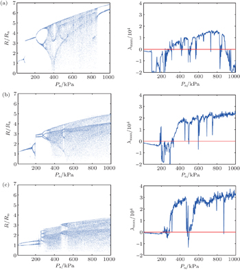
 | Fig. 1. Acoustic pressure amplitude bifurcation diagrams and Lyapunov exponent curves in the cases of (a) driving frequency va = 0.5 f0, (b) va = f0, and (c) va = 2 f0. |
Two different representations of the same oscillation are given in a row. There are, from left to right, acoustic pressure amplitude bifurcation diagrams, Lyapunov exponent curves. In the left row, there are the bifurcation diagrams with a fully developed period doubling cascading to chaotic oscillation for different acoustic frequencies. In the right row, there are the associated largest Lyapunov exponent λmax curves. The maximum Lyapunov exponent λmax is lower than zero for periodic oscillations, being zero at period doubling bifurcation points, and larger than zero for chaotic oscillation.
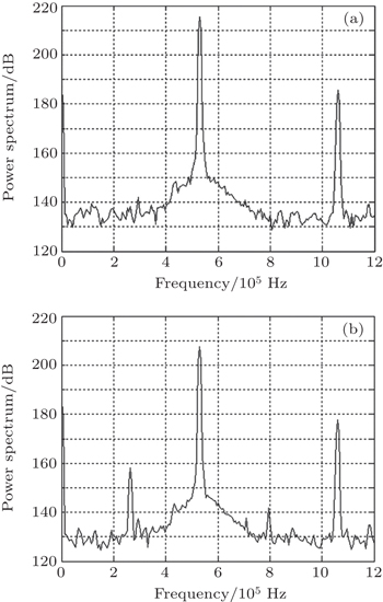
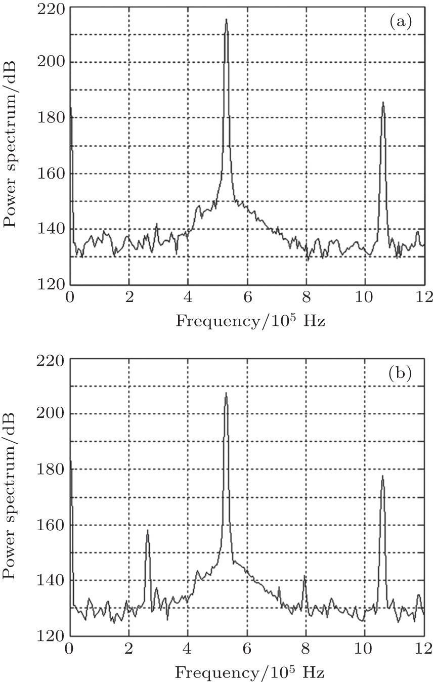 | Fig. 2. Power spectrum with send-receive distance of 0.3 m (a) without and (b) with bubbles. |
In the condition of typical bubble radius at rest Rn = 100 μm, it is shown that the dynamic characteristics of the system are more and more complex with the increasing of acoustic pressure amplitude. When acoustic pressure amplitude is above 100 kPa (220 dB), bifurcation appears, which represents that the system is in an unstable state. When acoustic pressure amplitude is between 600 kPa and 800 kPa (235.6 dB and 238.1 dB), the system is in chaotic state stably. Fixing the bubble radius at rest (resonance frequency is fixed), the acoustic pressure amplitude threshold of bifurcation is minimum when va = 2 f0 (Pa = 20 kPa).
An experiment is conducted in a water tank with dimensions of 1.5 m×1.2 m×1 m. The bubbles are generated by the method of water electrolysis, and its resonance frequency is about 80 kHz. When the bubble oscillations are driven by high-intensity single-frequency acoustic wave (acoustic pressure level achieves 200 dB), sub-harmonics in nonlinear system should appear. It is verified that sub-harmonics can appear when the excited acoustic pressure is not too high (as shown in Fig.
In this section, we present a summary of single bubble dynamics by means of Lyapunov exponent maps with respect to the driving pressure and frequency. This is to outline the critical role of the control parameters in bubble dynamics and to represent an outlook of the bubble dynamics complexity. The Lyapunov exponent map of an acoustically driven bubble is depicted in Fig.
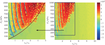
 | Fig. 3. Lyapunov exponent map of an acoustically driven bubble. The bubble radius at rest is Rn = 100 μm. The range of the studied frequency is from 0.1 f0 to 10 f0, and the pressure varies from 10 kPa to 1000 kPa. |
The map can be divided into two parts by a red color curve in the left of the figure. It is clearly shown that it is difficult to achieve the chaotic status when the normalized frequency is higher than 5. The system becomes extremely chaotic which maintains the whole remaining pressure interval between 750 kPa and 1000 kPa, where the normalized frequency va/v0 is between 2.5 to 5. In particular, there is a complex region in the left of the figure, where the the stable oscillation transforms into a chaotic one periodically. There are five gaps, which mean the stable oscillations between the regions of chaotic oscillations.
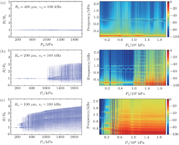
Oscillators are often described by frequency response curves, in which the frequency change is indicated. As is well known, the frequency response in a nonlinear system is much more complex than in a linear system. The frequency response curves for different bubble radii at rest driven by acoustic frequency va = 50 kHz, va = 100 kHz, va = 200 kHz, and va = 400 kHz are shown respectively in Figs.
When the linear resonance frequency of a bubble, f0, is much smaller than the driving frequency va, there exists a special frequency response, including bubble linear resonance frequency f0, excitation frequency va, Stokes frequency va − f0, and anti-Stokes frequency va + f0. This phenomenon is similar to the stimulated Raman scattering process in optics.
Frequency response diagrams can provide more details about the change of frequency component during the change of control parameter. With the increasing of acoustic pressure amplitude, more complex dynamics characteristics will arise, such as stimulated scattering, period-2, period-3, period-4, period-5, …, chaos, etc.
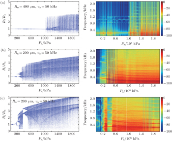
 | Fig. 4. Acoustic pressure amplitude bifurcation diagrams and frequency response diagrams versus acoustic pressure amplitude when driving frequency va = 50 kHz for (a) Rn = 400 μm (f0 = 8.823 kHz, and responding normalized frequency is 0.1764), (b) Rn = 200 μm (f0 = 17.673 kHz, and responding normalized frequency is 0.3534), and (c) Rn = 100 μm (f0 = 35.450 kHz, and normalized to 0.7090). |
 | Fig. 5. Acoustic pressure amplitude bifurcation diagrams and frequency response diagrams versus acoustic pressure amplitude when driving frequency va = 100 kHz for (a) Rn = 400 μm (f0 = 8.823kHz, and responding normalized frequency is 0.0882), (b) Rn = 200 μm (f0 = 17.673 kHz, and responding normalized frequency is 0.1767), and (c) Rn = 100 μm (f0 = 35.450 kHz, and normalized to 0.3545). |
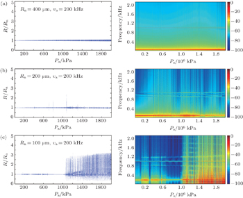
 | Fig. 6. Acoustic pressure amplitude bifurcation diagrams and frequency response diagrams versus acoustic pressure amplitude when driving frequency va =200 kHz for (a) Rn =400 μm (f0 = 8.823 kHz, and responding normalized frequency is 0.0441), (b) Rn =200 μm (f0 = 17.673 kHz, and responding normalized frequency is 0.0884), and (c) Rn =100 μm (f0 = 35.450 kHz, and normalized to 0.1772). |
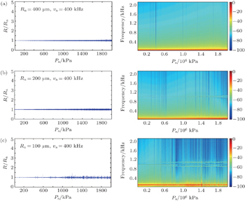
 | Fig. 7. Acoustic pressure amplitude bifurcation diagrams and frequency response diagrams versus acoustic pressure amplitude when driving frequency va = 400 kHz for (a) Rn = 400 μm (f0 = 8.823 kHz, and responding normalized frequency is 0.0221), (b) Rn = 200 μm (f0 = 17.673 kHz, and responding normalized frequency is 0.0442), and (c) Rn = 100 μm (f0 = 35.450 kHz, and normalized to 0.0886). |
It is shown that the stimulated sound scattering process happens much more easily when the linear resonance frequency of a bubble f0 is much smaller than the driving frequency va. There exist two additional frequency components increasing or decreasing near the driving frequency va stably. These are special phenomena in the process of stimulated sound scattering on a bubble due to the nonlinear interaction between linear resonance frequency and driving frequency. The two frequency components are Stokes component (its frequency f− = va − f0) and anti-Stokes component (its frequency f+ = va + f0), respectively.
With the increasing of the linear resonance frequency of a bubble f0, it is much more difficult for the stimulated sound scattering to occur. The bifurcation and chaos may play an important role in the bubble oscillation.
Examples of the phenomenon of stimulated sound scattering are given above. The threshold of stimulated sound scattering is associated with three major parameters, i.e., the bubble radius at rest (linear resonance frequency of bubble), acoustic frequency, and acoustic pressure amplitude. The threshold is much smaller when the ratio f0/va is not close to 1, meanwhile the Pa is not too big. On the one hand, when the f0 is close to va, the bifurcation may arise easily. On the other hand, with the increasing of Pa, the nonlinear resonance of a bubble may be destroyed by the state of chaos.
It is shown that the threshold of stimulated sound scattering is smaller than the ones of bifurcation and chaos in the common condition. When the bubble radius at rest decreases from Rn = 400 μm to Rn = 100 μm, the phenomenon of stimulated sound scattering gradually disappears as acoustic pressure amplitude increases. The interesting phenomenon shows that the bigger the bubble radius at rest, the larger the range of stimulated sound scattering is. For example, the phenomenon stimulated sound scattering will exist until Pa = 2000 kPa for Rn = 400 μm, but the phenomenon can only exist till Rn = 100 μm. On the other hand, it is easy to find out that the smaller the bubble radius at rest, the lower the acoustic pressure amplitude threshold from the bifurcation diagrams is. The system is not chaotic even when the driving amplitude achieves Pa = 200 kPa when the bubble radius at rest Rn = 400 μm. The threshold of chaos for Rn = 200 μm is about 100 kPa. However, in the condition of Rn = 100 μm, the system gradually comes into bifurcation only at Pa = 20 kPa.
Stimulated sound scattering is a special phenomenon which is associated with bubble nonlinear oscillation. Stimulated sound scattering is different from bifurcation and chaos, which is the result of the nonlinear resonance of a bubble under the excitation of high-amplitude acoustic sound wave essentially.
There is no doubt that the frequency responses of the system are complex versus acoustic pressure amplitude. The further research will focus on the variation of driving frequency, then we can obtain more detailed information about the evolution of this bubble oscillation system.
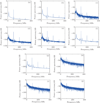
From the acoustic pressure amplitude-normalized frequency plane in frequency response diagrams, it is obvious that the frequency response of the system relies on the acoustic pressure amplitude. The power spectrum is a common method to characterize a nonlinear oscillation by its spectral content. Figure
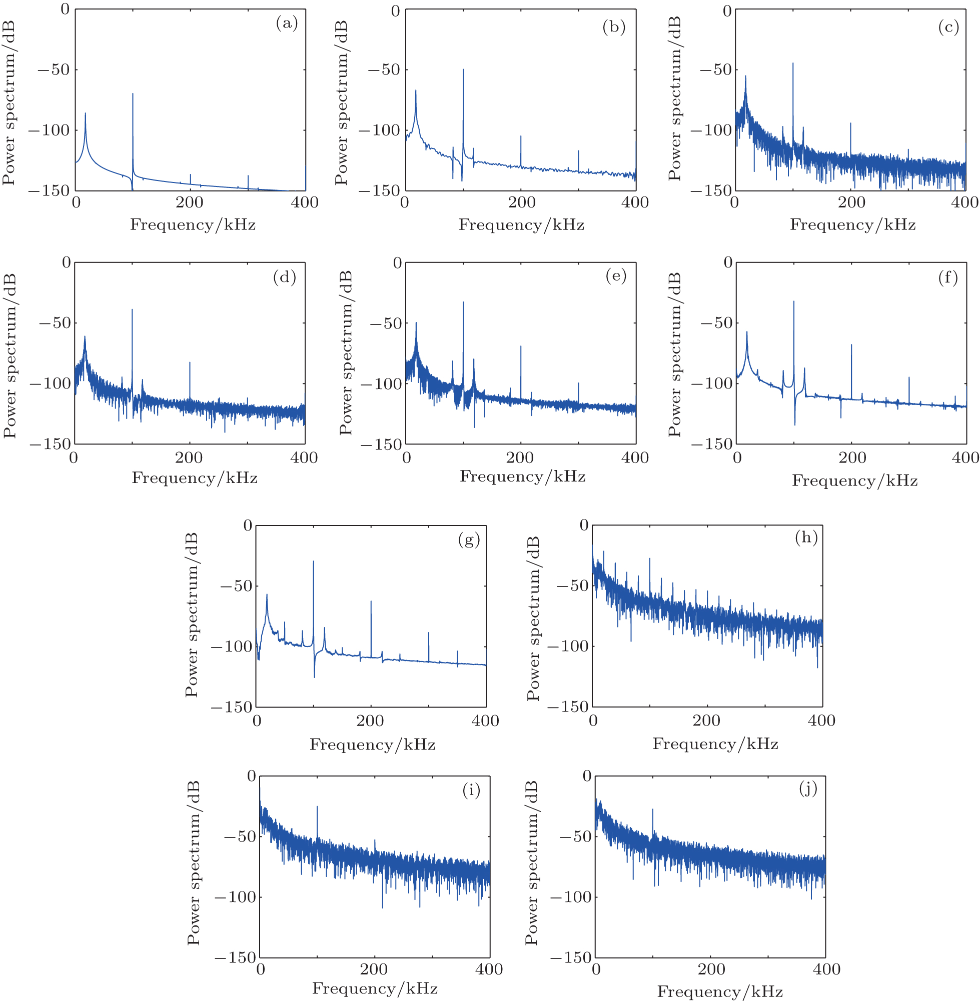 | Fig. 8. Power spectrum diagrams of the oscillation system response versus acoustic pressure amplitude at (a) Pa = 10 kPa (200 dB), (b) Pa = 100 kPa (220 dB), (c) Pa = 180 kPa (225 dB), (d) Pa = 350 kPa (230 dB), (e) Pa = 700 kPa (237 dB), (f) Pa = 750 kPa (237.5 dB), (g) Pa = 1000 kPa (240 dB), (k) Pa = 1400 kPa (242 dB), (i) Pa = 2000 kPa (246 dB), and (j) Pa = 2500 kPa (248 dB). |
When the acoustic pressure amplitude Pa = 200 dB, besides the driving frequency and its harmonics, there is only linear frequency response component in the system. When the driving amplitude reaches 220 dB, the special components, i.e., Stokes component and the anti-Stokes component arise, and the amplitudes of all the components increase as acoustic pressure amplitude increases. In the case of driving amplitude Pa = 237 dB, the system comes into period 5. Subharmonic components arise till Pa = 240 dB in the system, which shows that the system comes into bifurcation. With further increasing Pa, the frequency response of the system becomes more and more complex. When the amplitude achieves 248dB, the system is already chaotic. It looks like a noise spectrum. With the same excitation frequency, the oscillation can reach different states, such as stimulated scattering, period-2, period-4, period-5, …, chaos, etc.
In this article, the nonlinear dynamics of an acoustically excited gas bubble in water is investigated by theoretical and numerical analysis methods. The evolution of the bubble radius with time is modeled by using the Keller–Miksis equation, which takes into account the compressibility of the liquid. Our results show the bubble radius has strongly nonlinear behavior with respect to the pressure amplitude and excitation frequency as the control parameters, and give an intuitive insight into stimulated sound scattering on a bubble.
On the one hand, the Jacobian matrix is derived for calculating Lyapunov exponent, and the threshold values of chaotic motion under the periodic perturbation are obtained by using Melnikov’s method. The numerical simulations not only show the consistence with the theoretical analysis but also exhibit the bifurcation diagrams and Lyapunov exponent maps, which help to determine the chaotic states under many control parameters.
On the other hand, stimulated sound scattering is a special phenomenon which is associated with bubble nonlinear oscillation. Based on the Keller–Miksis equation, the phenomenon and threshold of stimulated sound scattering can be obtained by using a numerical analysis method and frequency response diagrams. The stimulated sound scattering is different from common dynamical behaviors, such as bifurcation and chaos, which is the consequence of the nonlinear resonance of a bubble under the excitation of high-amplitude acoustic sound wave essentially. The numerical analysis results show that the threshold of stimulated sound scattering is smaller than the ones of bifurcation and chaos in the common condition.
| 1 | |
| 2 | |
| 3 | |
| 4 | |
| 5 | |
| 6 | |
| 7 | |
| 8 | |
| 9 | |
| 10 | |
| 11 | |
| 12 | |
| 13 | |
| 14 | |
| 15 | |
| 16 | |
| 17 | |
| 18 | |
| 19 | |
| 20 | |
| 21 | |
| 22 | |
| 23 |