


Experimental and numerical studies of nonlinear ultrasonic responses on plastic deformation in weld joints
[Xiang Yan-Xun1, Zhu Wu-Jun1, Deng Ming-Xi2, Xuan Fu-Zhen1, †,  ]
]
]
|
|


† Corresponding author. E-mail:
Project supported by the National Natural Science Foundation of China (Grant Nos. 51325504, 11474093, and 11474361) and the Shanghai Rising-Star Program, China (Grant No. 14QA1401200).
The experimental measurements and numerical simulations are performed to study ultrasonic nonlinear responses from the plastic deformation in weld joints. The ultrasonic nonlinear signals are measured in the plastic deformed 30Cr2Ni4MoV specimens, and the results show that the nonlinear parameter monotonically increases with the plastic strain, and that the variation of nonlinear parameter in the weld region is maximal compared with those in the heat-affected zone and base regions. Microscopic images relating to the microstructure evolution of the weld region are studied to reveal that the change of nonlinear parameter is mainly attributed to dislocation evolutions in the process of plastic deformation loading. Meanwhile, the finite element model is developed to investigate nonlinear behaviors of ultrasonic waves propagating in a plastic deformed material based on the nonlinear stress–strain constitutive relationship in a medium. Moreover, a pinned string model is adopted to simulate dislocation evolution during plastic damages. The simulation and experimental results show that they are in good consistency with each other, and reveal a rising acoustic nonlinearity due to the variations of dislocation length and density and the resulting stress concentration.
Weld joints have been widely applied in pressure vessels, power plants, petrochemical industry, etc., which usually experience plastic damage, micro-crack initiation and growth due to the harsh service conditions in practice. Premature failures at weld joints have recently become a worldwide issue in engineering steels.[1] This failure occurs with the accumulation of cyclic plastic deformation which is generally accompanied with microstructure evolution in a material, such as dislocation multiplication, annihilation and sub-grain initiation. In order to identify the plastic damage and then evaluate the structural health, it is of increasing importance to track the microstructural evolution and then to evaluate the plastic damage of weld joints at an earlier stage. Nondestructive testing and evaluation (NDT & E) techniques such as ultrasonics, eddy-current, thermography, etc. are usually used for the quality assessment of the weld joints.[2] Recently, a nonlinear ultrasonic technique has emerged as a promising tool for NDT & E of the material property degradation,[3–21] such as fatigue, plastic damage, creep, and thermal damage. These references show that the response in harmonics generation can be related to the microstructural change in material.
Now there have been many reports on material assessment of fatigue or plastic deformation using second harmonic generation measurements of ultrasound.[3–21] The influence of a fatigue crack on the harmonic generation was first considered at unbounded interfaces,[7] where the results indicate that the variation of harmonic amplitude could be useful to monitor the state of fatigue. Then, a number of investigators have used nonlinear ultrasonic techniques to assess fatigue damage in different materials, such as plastics and composites,[8] stainless steel,[9] and aluminum alloy.[10] In recent years, there were generally three aspects attracting the attention of fatigue or plastic damage assessment using second harmonic generation measurements. First, various wave types such as surface acoustic wave[11,12] and Lamb waves[13–15] have been used for characterizing the fatigue damage in materials. Second, more exquisite and robust measurement methods such as air-coupled detection[16] have been adopted for ultrasonic measurements. Finally, more analyses of the relationship between second harmonic generation and fatigue/plastic deformation have been presented based on microstructural contributions, including some dislocation-dependent models[17–19] and micrograph-dependent analyses.[20,21] Though recently some investigations of fatigue or plastic deformation in various metallic alloys have been conducted by using nonlinear ultrasound, the systematic work and analysis on plastic damage in complex weld joints are still lacking. Compared with homogeneous materials, e.g. aluminum alloy and titanium alloy, the weld joints have very complex structure, which are more liable to suffer the damage induced by the fatigue/plastic loading.
In addition, most of the previous research focused on the experimental measurements of ultrasonic harmonic generation[11–16] and on the theoretical analyses mainly based on the dislocation monopole model,[22] the dislocation dipole model[10] and other improved models.[18,19] However, less information is available about the numerical analysis of nonlinear ultrasonic response from a damaged material. In fact, numerical simulation could help to provide some valuable insights into the relationship between the nonlinear ultrasonic responses and the degradation of materials. There are some numerical methods available to simulate nonlinearities of media and/or damage, such as finite element method (FEM),[23] finite difference time domain method (FDTD),[24] and local interaction simulation approach (LISA),[25] etc.
In this work, stress-controlled and strain-controlled tensile tests of 30Cr2Ni4MoV martensite weld joints are conducted for fabricating specimens with different plastic deformations, which then are evaluated by the nonlinear ultrasonic technique. The influence of microstructure evolution on the nonlinear ultrasonic responses is also thoroughly analyzed based on metallographic studies, such as transmission electron microscope (TEM). Finally, the commercial finite element analysis software Abaqus is used to simulate the nonlinear ultrasonic waves propagating in the weld region and to verify the correlation between microstructural evolution and the nonlinear ultrasonic measurement.
A martensite stainless steel 30Cr2Ni4MoV is used in the study, whose nominal chemical compositions in wt% are listed in Table
| Table 1. Chemical compositions of 30Cr2Ni4MoV stainless steel in wt%. . |
 | Fig. 1. Dimensions of flat dog-bone specimen of weld joint. All dimensions are in unit mm. |
Two sets of plastic deformed specimens are made for experiments using a 100-kN MTS servo hydraulic testing system. One group with 7 specimens are fabricated under stress-controlled mode loading from 774 MPa to 869 MPa (yield strength is 785 MPa), and another one with 5 specimens are fabricated under strain-controlled mode from strain levels of 1.14% to 3.89%. The nonlinear ultrasonic measurements are made off-line after unloading the specimens.
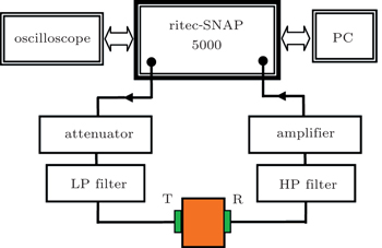
Nonlinear ultrasonic measurements are performed on three locations of the specimens, i.e., weld region (about 20 mm in the center), HAZ region (about 2 mm nearing the weld), and the base region. For nonlinear ultrasonic measurement, a Ritec SNAP system with model of RAM-5000 is used to generate the ultrasonic signal. The experimental setup for longitudinal wave measurement is illustrated in Fig.
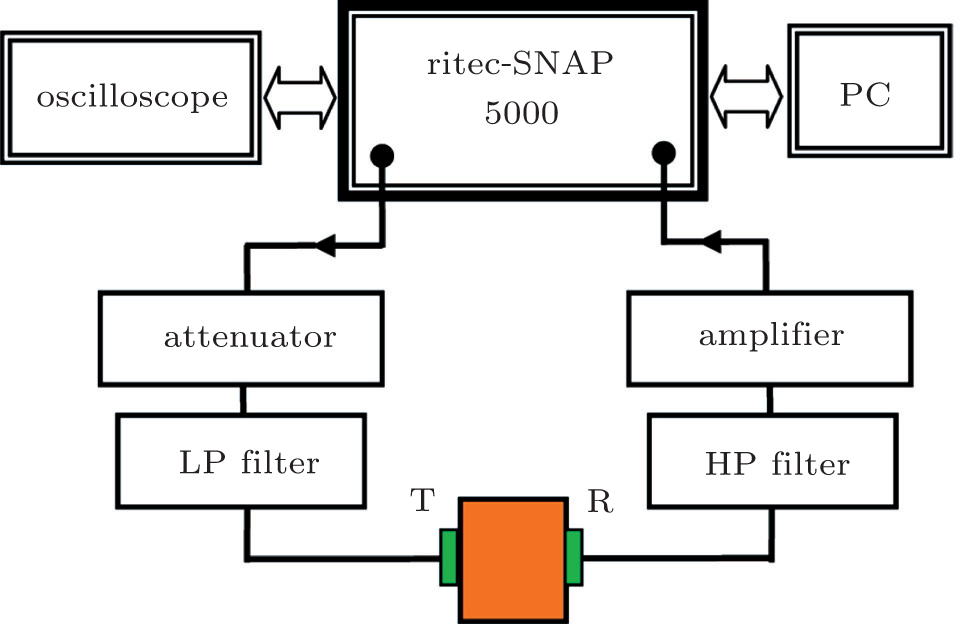 | Fig. 2. Experimental setup for nonlinear ultrasonic measurements.[3] |
When exciting a sample by using a single frequency excitation, the second-order nonlinear parameter, known as β, generated by the presence of damaged structure can be expressed as


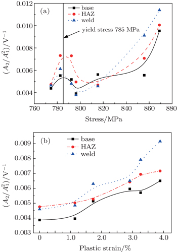
Figures 
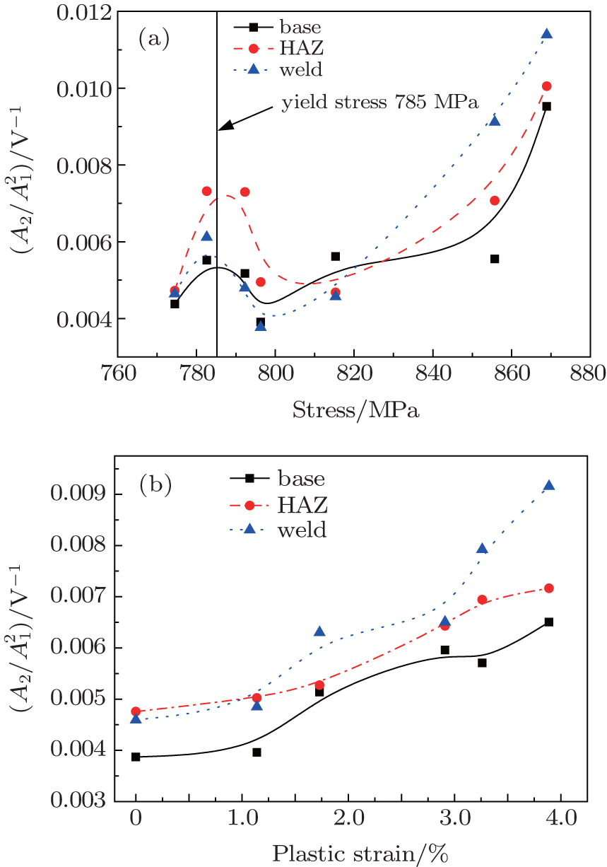 | Fig. 3. Variations of the RANP |
Microstructure changes of the martensite steel subjected to plastic deformation are thought to originate from the variation of acoustic nonlinearity.[17] Therefore, TEM are used to observe the microstructural evolutions and understand the change of the
Figure
| Table 2. Microstructure parameters of 30Cr2Ni4MoV weld joint specimens with different plastic strains. . |
 | Fig. 4. TEM micrographs of 30Cr2Ni4MoV weld joint specimens with different plastic strain levels: (a) virginal specimen; (b) 1.14% plastic strain; (c) 1.73% plastic strain, and (d) 3.89% plastic strain.[3] |
Finite element simulations are now presented to assist in explaining the experimental results. Consider an isotropic homogeneous solid medium with purely elastic behavior, the nonlinearities of the medium which would contribute to the acoustic nonlinearity may originate from different sources, such as the material and geometric nonlinearities, fatigue- or stress-induced plasticity, etc.
Considering the longitudinal waves in the medium and ignoring the dispersion and attenuation, the equations of motion in the Lagrangian coordinate

The stress tensor in Eq. (


Considering a one-dimensional medium such as a rod, the wave solution of Eq. (


For a medium experiencing plastic deformation, localized plasticity damage would appear in the form of microstructural defects such as dislocations, which could be a source of nonlinearity for the wave propagation. In contrast to βI, another nonlinearity parameter βD is defined to describe the plasticity-induced nonlinearity for the damage state of the material. For ease of numerical simulation, here we restrict discussion to the dislocation monopoles contributing to the nonlinear parameters of the material, which can be expressed as[22,30]


Therefore, the acoustic nonlinearity parameter β of Eq. (
Based on the above analyses of the nonlinear elastodynamics, a finite element simulation is conducted in an attempt to explain the variation of acoustic nonlinearity in the plasticity deformed material, which is developed and carried out on the basis of the commercial FEM software Abaqus/EXPLICIT. The intact state and plastic-damaged state with dislocations in materials are taken into account in the following FEM models.
The numerical simulation of material, geometric, and plasticity-induced nonlinearities is performed by introducing the nonlinear stress-strain constitutive relation (i.e., Eq. (
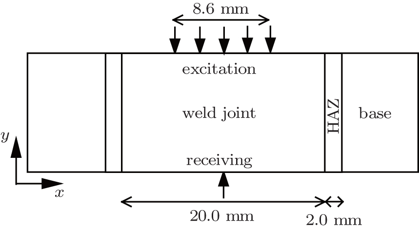 | Fig. 5. Schematic diagram of the simulation model for longitudinal wave propagating in weld joint. |
The four-node reduced-integration plane strain elements (CPE4R) in Abaqus are used to mesh the rectangular model through a structured meshing algorithm, whose elements are equally sized at 0.05 mm (Δy) with a spatial resolution of λL/24 where λL is the wavelength of the fundamental wave (about 1.2 mm). This spatial resolution is chosen to warrant simulation precision and error convergence. According to the Fourier or von Neumann stability analysis,[32] the time step Δt should be smaller than the time required for the longitudinal wave to travel across the element length, that is,

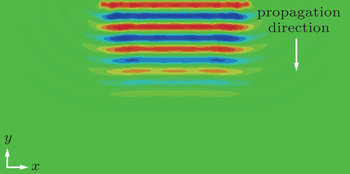
A snapshot of the ultrasonic wave (in the form of stress contour) propagating in the weld joint is shown in Fig.
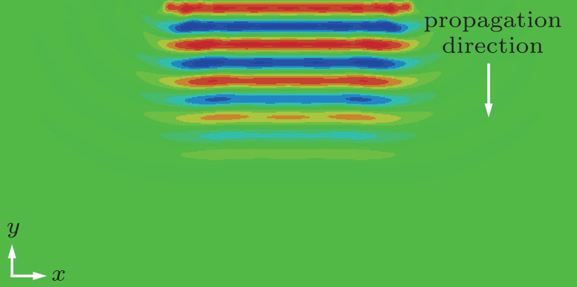 | Fig. 6. A snapshot of the ultrasonic wave propagating in the weld joint (in the form of stress contour). |
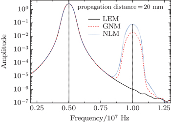
According to the above different conditions of (i)–(iii), figure
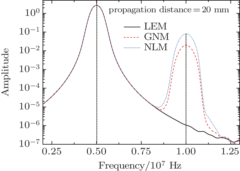 | Fig. 7. Frequency domain signals obtained using LEM, GNM, and NLM stress–strain constitutive models. |
Prior to the numerical simulations, some assumptions should be made for the simulations of plastic-damaged state with dislocations in material. First, only plastic-induced edge dislocations are taken into account in the following simulations just as shown in Fig.
It can be seen from the microstructural analysis of Subsection 2.3 and Table
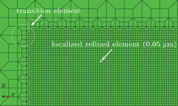
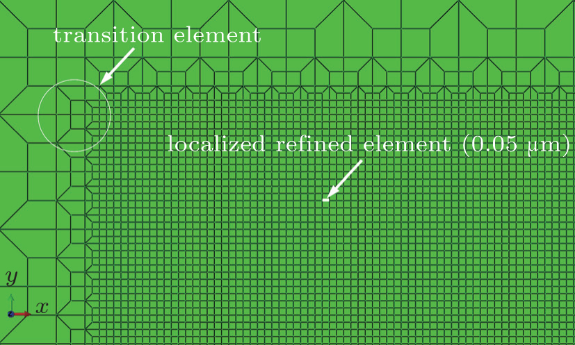 | Fig. 8. Meshed structure with localized refined mesh (LRM) and a minimum element length of 0.05 μm formed by using transition element. |
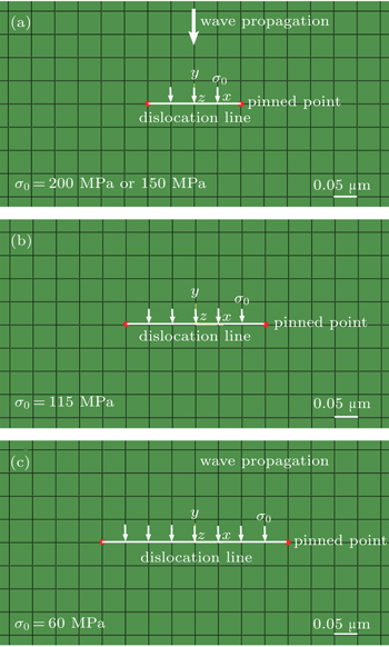
Three examples of numerical simulations for dislocations with different pinned lengths such as 0.2 μm, 0.3 μm, and 0.4 μm are demonstrated, corresponding to the really measured dislocation lengths as given in Table
 | Fig. 9. configurations of the dislocation located in the middle of the LRM model, in which pinned strings are used for modeling different dislocations in the damaged states: (a) 0.2 μm, (b) 0.3 μm, and (c) 0.4 μm. The solid circles represent the pinned points of dislocations with a zero displacement. |
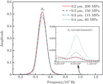
Figure
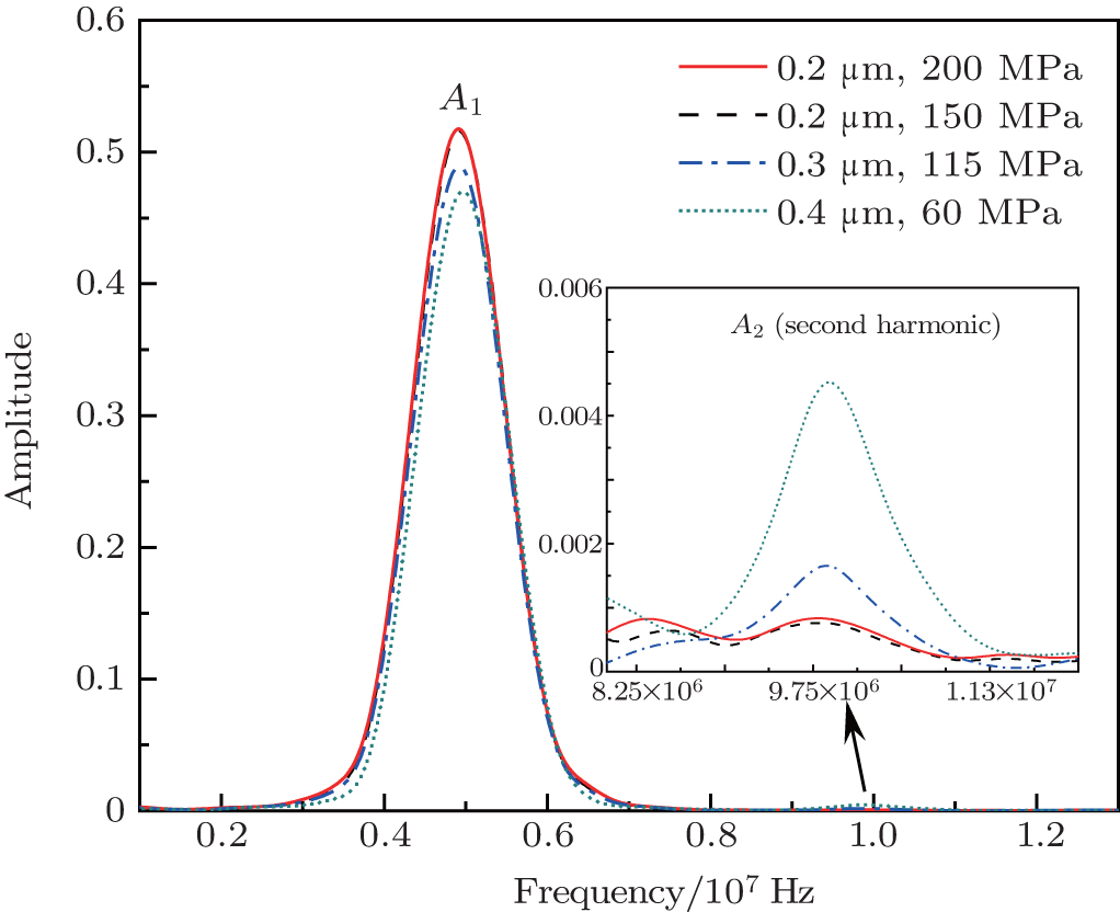 | Fig. 10. Amplitudes of the fundamental (A1) and second-harmonic (A2) in the frequency domain for simulation of dislocations with different lengths. |
| Table 3. Values of dislocation simulation for the plastic deformed materials. . |
From Figs.
Note that the above established LRM model represents the damaged state only with one dislocation. Here, in order to extend a one-dislocation result into multi-dislocation state to simulate the practical specimens conducted in the experiments, we can make a correlation of βD with the simulation result of one-dislocation
Then, the term on the right-hand side of Eq. (
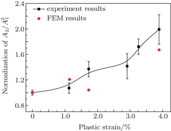
Figure
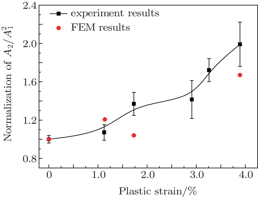 | Fig. 11. Normalized |
However, the calculated results from the FEM model are underestimated compared with those measured results, especially in the late stage. In this perspective, there may be other microstructures that would contribute to the acoustic nonlinearity during the plastic strain loading, such as the dislocation cells or walls, as marked by arrows in Fig.
In this article the experimental measurement and numerical simulation are performed to study the ultrasonic nonlinear responses from the plastic deformation in 30Cr2Ni4MoV weld joints. The measurement results show that the normalized nonlinear parameter
Meanwhile, an FEM model is presented to investigate the behavior of nonlinear wave propagation associated with material and plastic damage, which is carried out by introducing the nonlinear stress-strain constitutive relation to Abaqus through the interface of user subroutine VUMAT. The modeling technique focuses on material, geometric and plasticity-induced nonlinearities that may contribute to the variation of acoustic nonlinearity. A pinned string model is used to simulate dislocation evolution (0.2 μm–0.4 μm) during the plastic damage. Results from the simulation and the experiments show that they are in good consistency with each other, both reveal a rising acoustic nonlinearity due to the variation of the dislocation length and density. The FEM model developed here could be a good supplementary way to provide insights into the nonlinear wave propagation and its interaction with the dislocations, precipitates and micro-voids or micro-cracks in materials.
| 1 | |
| 2 | |
| 3 | |
| 4 | |
| 5 | |
| 6 | |
| 7 | |
| 8 | |
| 9 | |
| 10 | |
| 11 | |
| 12 | |
| 13 | |
| 14 | |
| 15 | |
| 16 | |
| 17 | |
| 18 | |
| 19 | |
| 20 | |
| 21 | |
| 22 | |
| 23 | |
| 24 | |
| 25 | |
| 26 | |
| 27 | |
| 28 | |
| 29 | |
| 30 | |
| 31 | |
| 32 |