Property of slice square polycapillary x-ray optics
Peng Shi-Qi1, 2, 3, Liu Zhi-Guo1, 2, 3, †, , Sun Tian-Xi1, 2, 3, Wang Kai1, 2, 3, Yi Long-Tao1, 2, 3, Yang Kui1, 2, 3, Chen Man1, 2, 3, Wang Jin-Bang1, 2, 3
The Key Laboratory of Beam Technology and Material Modification of the Ministry of Education, Beijing Normal University, Beijing 100875, China
College of Nuclear Science and Technology, Beijing Normal University, Beijing 100875, China
Beijing Radiation Center, Beijing 100875, China


† Corresponding author. E-mail: liuzhiguo512@126.com

Project supported by the Fundamental Research Funds for the Central Universities, China (Grant Nos. 2012LZD07 and 2014kJJCA03) and the National Natural Science Foundation of China (Grant Nos. 11375027 and 11075017).

Abstract
Abstract

A geometrical description of square polycapillary x-ray optics and the basic theory of the transmission of x-rays are presented. A method of numerical calculation is developed based on ray-tracing theory. The method simulates the intensity distribution of x-rays propagating through slice square polycapillary x-ray optics. The simulation results are compared with the experimental results.

1. Introduction

Slice square polycapillary x-ray optics has been studied for more than a decade[14] and has attracted increasing attention recently.[5,6] Square pores arrange regularly in the slice square polycapillary x-ray optics. In flat slices, rays undergoing reflections at grazing incidence from two orthogonal walls will have both their direction cosines reversed, which enables point-to-point focusing of a source, which means that the source distance and the image distance are equal, i.e., f1 = f2. As to the slumped slices, this kind of optic can be used to convert the diverging beam from a point-like source at its focus into a quasi-parallel output beam, or conversely, converge the parallel beam. Usually, this kind of optics is used in the area of x-ray imaging, so its focal spot size is not taken into consideration in this paper. If there are no channel misalignments happening during the manufacturing process, the shape of the focal spot is a cross with no defect. So the shape of the focal spot is considered as a criterion to evaluate the quality of the arrangement of the channels in the slice square polycapillary x-ray optics.

In this paper, a simulation model is presented, a method is presented to establish a geometrical model of the slice square polycapillary x-ray optics. Simulation results based on this model are compared with the experimental results, and the influence of the channel misalignments is also demonstrated.

2. Experiment
2.1. Experimental arrangements

The test optic is flat slice square polycapillary x-ray optics, which has a large 20 mm×20 mm planar format, comprised of square-packed channel multifibers. The channel side-length is 20 μm, and the mean thickness of the channel wall is 3.91 μm. X-rays are generated by a Cu target x-ray tube with a 25-kV source voltage and its focal spot size is 50 μm.

As the slice square polycapillary x-ray optics in this experiment is flat, it will focus x-rays in a point-to-point manner. It is thus mounted in a two-axis carriage at the midpoint of the beam line as shown in Fig. 1. The source-optic and optic-image distances are f1 = f2 = 500 mm.

Fig. 1. Schematic view of the experimental arrangement.
2.2. Experimental results

An image (Fig. 2(a)) of the slice square polycapillary x-ray optics focus is recorded by using HAMAMATSU M1127-61 with a pixel size of 10 μm. A cross can be seen clearly in the image, but the cross broke into several sections. This is because of the channel misalignments which happen in its manufacturing process.

Fig. 2. (a) Image recorded by the digital camera; (b) some channels in the slice square polycapillary x-ray optics tilt to a small angle in their manufacturing process; (c) some channels in the slice square polycapillary x-ray optics move a small distance during their manufacturing process.

One kind of misalignment is called “tilting”, some channel layers tilt to a small angle in their manufacturing process (see Fig. 2(b)), and the error caused by this is termed “tilting error”. Another kind of misalignment usually happening in the manufacturing process is called “dislocation” (see Fig. 2(c)), and the error caused by this is referred to as “dislocation error”. To find out the influences of these two kinds of misalignments on the light spot and help to adjust the manufacturing process, some simulations are performed.

3. Modelling
3.1. Ray-tracing theory

An x-ray is a kind of electromagnetic wave which has relatively high energy; it can be reflected from the surface of a material if its glancing incidence angle is less than a value that is called the critical angle θc. Because the energy loss of this type of reflection is very small, the reflection can be regarded approximately as total reflection.

The critical angle is a function of photon energy and material itself; usually, the critical angle for total reflection of x-rays can be written as[7]

where Ek is the photon energy (in unit keV).

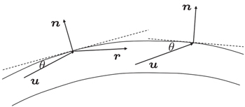
Assume that and are unit vectors in the directions of the incident and reflected beams, respectively, and is the unit vector normal to the inner wall of channel. As shown in Fig. 3, the glancing incidence angleθ = sin–1(n × r). If, the x-ray is totally reflected, and the reflected vector can be expressed as = –2sinθ. Otherwise, the x-ray will be absorbed by the inner wall.

Fig. 3. Diagram of the ray-tracing method.
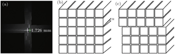
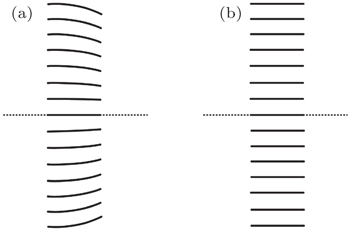
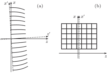
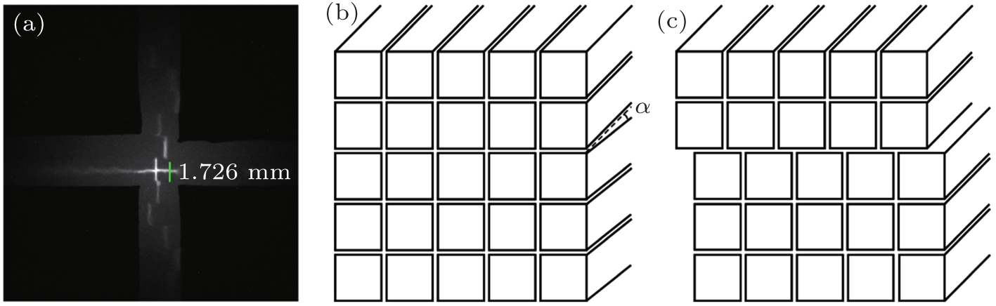
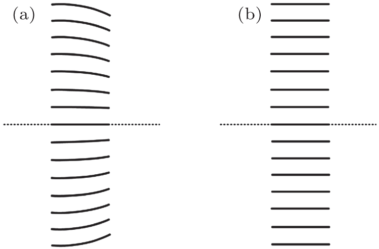
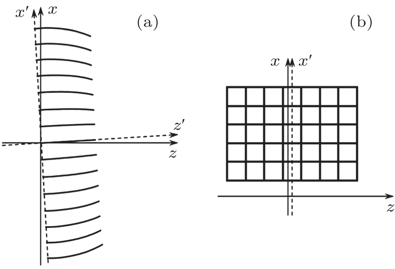
3.2. Model of the slice square polycapillary x-ray optics

If the tangents to the edges of all the channels point to a fixed point on the central axis of the slice, then the optic can focus rays from infinity (see Fig. 4(a)), and in this case the center line of each channel inside can be given approximately by fn(z) = anz2 + bnz + cn, and this kind of optics is called “slumped slice”. If the center line of each channel is parallel to the center line of the slice (see Fig. 4(b)) then an = 0, bn = 0, and this kind of optics is termed “flat slice”. Each channel in the slice consists of four walls. To realize the ray-tracing process, equations to express these walls must be established.

Fig. 4. (a) Slumped slice, (b) flat slice.

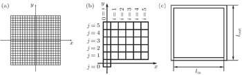
Cross-section of the slice square polycapillary x-ray optics can be seen in Fig. 5(a), among all those channels, channels in the first quartile (see Fig. 5(b)) need to be addressed first, and the geometrical characteristics of the remainder can be found by rotating the coordinate axis. Defining the channel in the center as layer zero (i = 0, j = 0), there are in total n layers in the square lens. Assume that the external wall of the outermost layer of channels can be fit by the function f(z) = a0z2 + b0z + c0. It is not difficult to show that for the channel in row j and column i, the external walls can be expressed by four equations. The top wall is expressed as

its bottom wall can be given as

its left-side wall is expressed by

the right-side wall is

Fig. 5. (a) Cross-section of the slice square polycapillary x-ray optics; (b) area of interest of the slice square polycapillary x-ray optics; (c) the cross-section of a square channel.

The thickness of the channel wall cannot be ignored; therefore we also impose the condition that the ratio between internal and external side lengths of the channel is fixed to be 0.8 (see Fig. 5(c)). Thus, the internal wall of the channel can be described by the following four equations:

Those four equations can be simplified into

As the projection of the vector normal to the upper wall on the y axis is positive, it can be deduced that the unit vector normal to the upper wall can be given as

where mx = 0, my = 1, and mz = –2auzbu.

For the lower wall, the projection of its normal vector on the y axis is negative; it is easy to show that mx = 0, my = –1, and mz = 2auz + bu.

Accordingly, for the left-side wall, we have mx = –1, my = 0, and mz = 2auz + bu.

For the right-side wall, we have mx = 1, my = 0, and mz = –2auzbu.

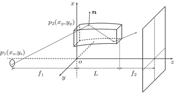
Let p1 be a point on the source whose coordinates are (xs,ys,zs) and p2 be a point on the channel entrance whose coordinates are (xp,yp,zp) (see Fig. 6), then the incident light ray will be determined by these two points, and the unit vector in this direction is

where d0 is the distance between the two points, which is given by

The glancing angle is

Thus, the reflected direction can be expressed by

Noting that the reflected x-ray is the next incident ray, an iteration procedure can be used to find its trajectory.

Fig. 6. Diagram of x-ray transmission in a channel.

Another important part in the mathematical model is to find the intersection point of the beam with the channel inner wall. Assuming that the starting point of an incident ray is (xs, ys, zs), and the end point is (xc, yc, zc), it is easy to see that the end point is the intersection point. Then, the line of the incident ray is given by

The substitution of Eq. (13) into Eq. (7) will give another four quadratic equations whose roots can be resolved through the quadratic formula. At least two real roots can be extracted. Roots with values larger than zs should be considered to be reasonable, and among them, the minimal root is the one corresponding to the intersection point.

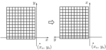
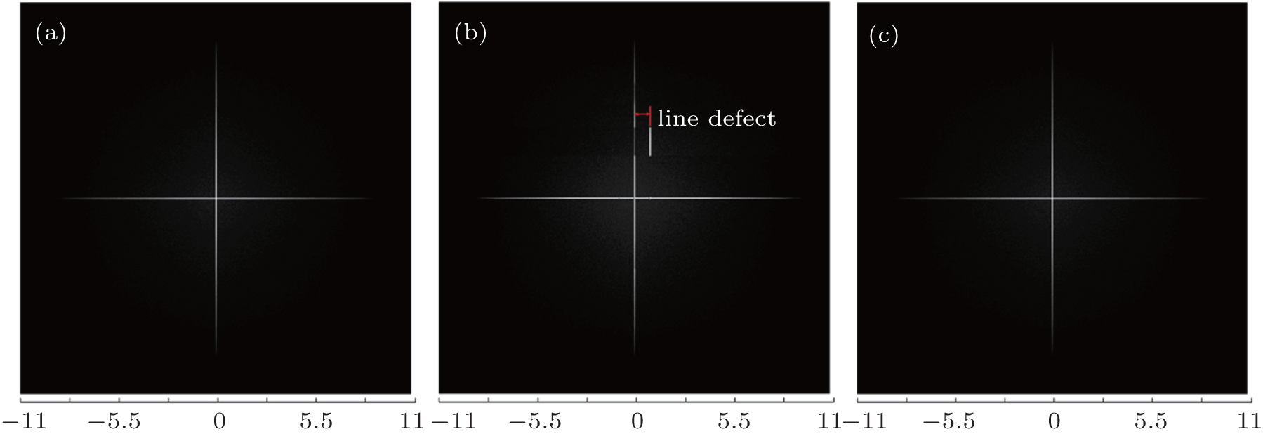
As for the channels in other quadrants, the method of rotating the coordinate axis can be used to establish their geometric model and study their transmission characteristics. Once the point (xs, ys) is chosen, rotate the coordinate axis and transform the channels into the first quadrant (see Fig. 7); then calculate the new coordinates of the point (xs, ys). After the iteration process, rotate the coordinate axis back to determine the coordinates of the emergent beam across the imaging plane.

Fig. 7. Demonstration of rotating the coordinate axis.
3.3. Simulation of the beam intensity distribution

We choose N points on the source at random. We then use a ray-tracing method to find the trajectories of rays and determine whether a ray could emerge from the exit. To find the intensity distribution of the emergent beam, the coordinates of beams crossing the imaging plane need to be known. Let the unit vector in the direction of the emergent light be un, the last total reflection point be (xsn, ysn, zsn), and the distance between the exit plane and the imaging plane be f, then the coordinates of the beam across the imaging plane will be

3.4. Tilting error and the dislocation error

In the manufacturing process, misalignment is inevitable, so in this model misalignment must be taken into account. As to the tilting error, the method of rotating the coordinate axis is used again. Once the point (xs, ys) is chosen, rotate the coordinate axis until the center line of the channel is parallel to the z axis, then calculate the new coordinates of this point (see Fig. 8(a)). After the ray-tracing process, rotate the coordinate axis back. As to the dislocation error, shifting transformation of the coordinate is used. Once the point (xs, ys) is chosen, shift the coordinate to correct the dislocation (see Fig. 8(b)), and shift the coordinate back after the ray-tracing process.

Fig. 8. (a) Rotate the coordinate axis; (b) shift the coordinate axis.
4. Results and discussion

To demonstrate the capability of the model to simulate the beam transmitting in a slice square polycapillary x-ray optics, the simulation results of the intensity distribution of flat slices are shown in Fig. 9. In the simulation, a point source (which means that for each incident light ray the coordinate of p1 is (xs, ys, zs) constantly) and x-ray energy E = 8.05 keV are used. The parameters of the slice square polycapillary x-ray optics are L = 2 mm, Φ = 20 mm, f1 = 500 mm, f2 = 500 mm, and the number of layers n = 500. In Fig. 9(a), there is no misalignment; in Fig. 9(b), the channels from the 60th layer to the 100th layer all tilt to an angle of 0.1°, and in Fig. 9(c) the channels from the 60th layer to the 100th layer all move to the right 10 μm. In Fig. 9(a), a cross without defect is shown, and this is what the light spot should be if there is no misalignment.

Fig. 9. (a) Simulation result of the slice square polycapillary x-ray optics without tilting error; (b) simulation result of the slice square polycapillary x-ray optics with tilting error; (c) simulation result of the slice square polycapillary x-ray optics with dislocation error.

A broken cross is shown in Fig. 9(b), one segment of the cross moves a small distance because of the tilting error, and a notable similarity between the experimental and simulated images is clearly evident. The line defect in this condition is 1.75 mm. Figure 9(c) shows a cross the same as the one in Fig. 9(a), which means that the reason leading to the defect of the light spot is the tilting error, and the dislocation error plays little role.

To show the influence of the tilting error on the defect of the light spot, another two simulations are performed, in these two simulations the parameters are as follows: E = 8.05 keV, L = 2 mm, Φ = 20 mm, f1 = 500 mm, f2 = 500 mm, and the number of layers n = 500. The relationship between the tilting angle and the line defect is shown in Table 1.

Table 1.

Simulation results.

.
5. Conclusions

With ray-tracing methods and numerical calculations, intensity distributions of x-rays through a slice square polycapillary x-ray optics are simulated. The simulation results show that the real reason which causes the defect in the light spot is the tilting error not the dislocation error. These simulation results can be used for designing and manufacturing slice square polycapillary x-ray optics.

Reference
1Siegmund O H WMcPhate J BTremsin A SJelinsky S RFrisch H JElam J 2012 Phys. Proc. 37 803
2Siegmund O HWMcPhate JTremsin A SJelinsky S RHemphill RFrisch H J 2012 Nuclear Instruments and Methods in Physics Research Section A: Accelerators, Spectrometers, Detectors and Associated Equipment 695 168
3Price G JBrunton A NBeijersbergen M WFraser G WBavdaz MBoutot J PTomaselli E 2002 Nuclear Instruments and Methods in Physics Research Section A: Accelerators, Spectrometers, Detectors and Associated Equipment 490 276
4Satake S IKunugi TSato KIto TTaniguchi J 2005 Opt. Rev. 12 442
5Jiang H YRen Y KAo H RRamos A 2008 Chin. Phys. B 17 4541
6Siegmund O H 2004 Nuclear Instruments and Methods in Physics Research Section A: Accelerators, Spectrometers, Detectors and Associated Equipment 525 12
7Hampai DDabagov S BCappuccio GCibin G2005X-ray and Neutron Capillary Optics IIInternational Society for Optics and Photonics 594302–59430210.1117/12.640111