Sun Zheng, Ning Hui, Tang Jing, Xie Yong-Jie, Shi Peng-Fei, Wang Jian-Hua, Wang Ke. Anomalous propagation conditions of electromagnetic wave observed over Bosten Lake, China in July and August, 2014. Chinese Physics B, 2016, 25(2): 024101
Permissions
Anomalous propagation conditions of electromagnetic wave observed over Bosten Lake, China in July and August, 2014
Sun Zheng†, , Ning Hui, Tang Jing, Xie Yong-Jie, Shi Peng-Fei, Wang Jian-Hua, Wang Ke
Northwest Institute of Nuclear Technology, Xi’an 710024, China
Atmospheric duct is a common phenomenon over large bodies of water, and it can significantly affect the performance of many radio systems. In this paper, a two-month (in July and August, 2014) sounding experiment in ducting conditions over Bosten Lake was carried out at a littoral station (41.89° N, 87.22° E) with high resolution GPS radiosondes, and atmospheric ducts were observed for the first time in this area. During the two months, surface and surface-based ducts occurred frequently over the Lake. Strong diurnal variations in ducting characteristics were noticed in clear days. Ducting occurrence was found at its lowest in the early morning and at its highest (nearly 100%) in the afternoon. Duct strength was found increasing from early morning to forenoon, and reaching its maximum in the afternoon. But contrarily, duct altitude experienced a decrease in a clear day. Then the meteorological reasons for the variations were discussed in detail, turbulent bursting was a possible reason for the duct formation in the early morning and the prevailing lake-breeze front was the main reason in the afternoon. The propagation of electromagnetic wave in a ducting environment was also investigated. A ray-tracing framework based on Runge–Kutta method was proposed to assess the performance of radio systems, and the precise critical angle and grazing angle derived from the ray-tracing equations were provided. Finally, numerical investigations on the radar performance in the observed ducting environments have been carried out with high accuracy, which demonstrated that atmospheric ducts had made great impacts on the performance of radio systems. The range/height errors for radar measurement induced by refraction have also been presented, too, which shows that the height errors were very large for trapped rays when the total range was long enough.
As an anomalous propagation mechanism in the marine troposphere or above other large bodies of water, atmospheric ducts can significantly affect the electromagnetic wave (EMW) propagation from the UHF band to sub-millimeter wave, which would lead to some unexpected effects for radars, high power microwave (HPM), GPS, wireless communication systems, and so on, such as extending the maximum detection range of radars, enhancing radar clutter, creating radar holes (or shadow zone), and causing positioning errors.[1–3] So an accurate knowledge of the ducting information will be needed to assess the performance of radio systems, especially for radar and HPM.
Atmospheric duct frequently occurs over oceans, seas, and coastal areas all over the world where humidity decreases rapidly with altitude. The most famous ducting area is the Persian Gulf which is entirely surrounded by desert landmass. Lots of pages of scientific research about the local boundary layer conditions have been published until now.[3–5] In Europe and South Asia, the ducting conditions over the Baltic Sea,[6,7] the English Channel,[8,9] the Mediterranean region,[10] and the Indian Ocean[11] have been reported. As for China, lots of investigations have been made on the ducting conditions over the East China Sea and South China Sea during the last two decades.[12–16] In recent years, a ship-based ducting measurement both over the South China Sea and the Eastern Indian Ocean has been reported.[17] The horizontal inhomogeneity of evaporation ducts and their impact on the EMW propagation has also been reported.[18] However, previous researches were always focusing on the large seas around the world; fewer researches have been done with the endorheic lakes, especially for Qinghai Lake and Bosten Lake in China. In this paper, a short-term meteorological sounding experiment was carried out over Bosten Lake during July and August, 2014, and the clear-air ducting conditions over the Lake are shown for the first time. Then a ray tracing framework for modeling EMW propagation based on Runge–Kutta method is presented.
During the last two decades, although two new important techniques have been developed to determine ducts over large bodies of water, i.e., Simulated Model based on numerical weather prediction (NWP) techniques[18–20] and refractivity from radar clutter (RFC) technique,[21–24] there were some disadvantages about the two techniques. As showed by Guo X M et al.,[15] the predicted duct altitudes via NWP techniques were not so accurate compared with the direct measuring results. As for RFC technique, the accuracy of the estimated refractivity heavily depends on a priori information that given.[24] In this work, we would employ the conventional way using modern high-resolution GPS radiosonde to determine the vertical refractivity profiles over Bosten Lake, which will be shown in Section 2. The duct characteristics, i.e., ducting occurrence, duct strength, and layer thickness, will be shown in that section, as well as the diurnal variation of ducts. In Section 3, meteorological reasons for diurnal ducting variation will be given. In Section 4, we will present a ray tracing framework for modeling EMW propagation, and then a rigorous result about the EMW propagation characteristics in a ducting layer, i.e., critical angle and grazing angle, will be given. Finally, a simulating result of EMW propagation under the existed ducting environments over the Lake will be presented with high accuracy.
2. Ducting conditions over Bosten Lake
As one of the largest inland freshwater lakes of China, Bosten Lake, which is located in the southern part of Xinjiang Uygur Autonomous Region, covers an area of nearly 1200 km2, its maximum dimensions are about 56 km in length and 25 km in width, and the Lake surface is about 1048 m high above the sea level. It is entirely surrounded by Gobi-desert landmass, which is similar to the Persian Gulf, and a temperate desert climate prevails in the area all around generally. Previous studies stated that atmospheric ducts can be easily formed by advection of warm, dry air coming from the desert over cooler water,[4,5,25] thus from this point of view, the Lake is a high-occurrence ducting area theoretically. Ducting conditions predict negative vertical gradient of modified refractivity as a result of strong gradients of temperature and humidity in the atmosphere. The modified refractivity M is defined by the empirical equation
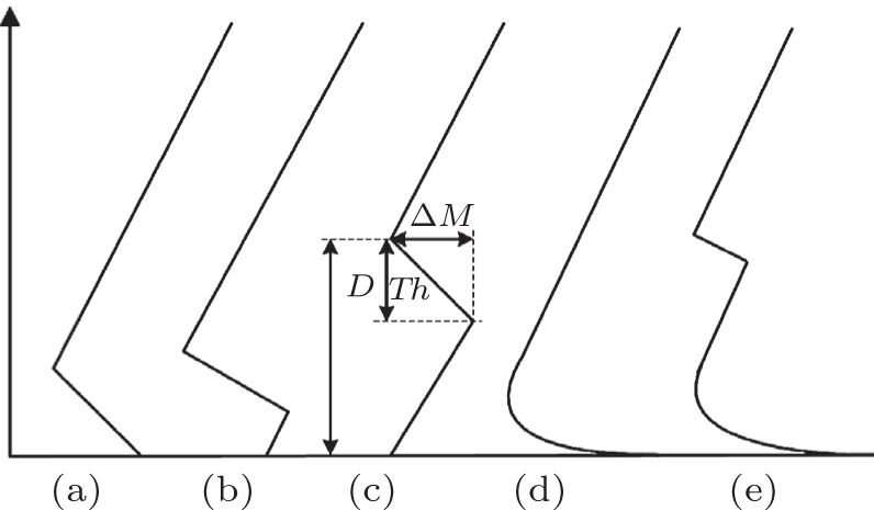
where P (in unit hPa) is the total atmospheric pressure; T (in unit K) is the atmospheric temperature; RH (in non-dimensional unit) is the relative humidity; es (in unit hPa) is the saturated pressure of water vapor at temperature T; z (in unit meter) is the height above the surface of the earth; and ae (in unit meter) is the local Earth’s effective radius. It is certain that the elevation height of a plateau lake should be taken into consideration for ae. The first two terms in Eq. (1) represent the refractivity N, and the additional term is the result of taking consideration of Earth’s curvature when modeling the EMW propagation. There exist several types of ducts, e.g., surface duct, surface-based duct, evaporation duct, elevated duct, and complex duct, which are illustrated in Fig. 1.
Fig. 1. Idealized M-profiles of (a) surface duct, (b) surface-based duct, (c) elevated duct, (d) evaporation duct, and (e) complex duct. The duct altitude D, duct thickness Th, and duct strength ΔM are illustrated on elevated duct.
2.1. Measurements
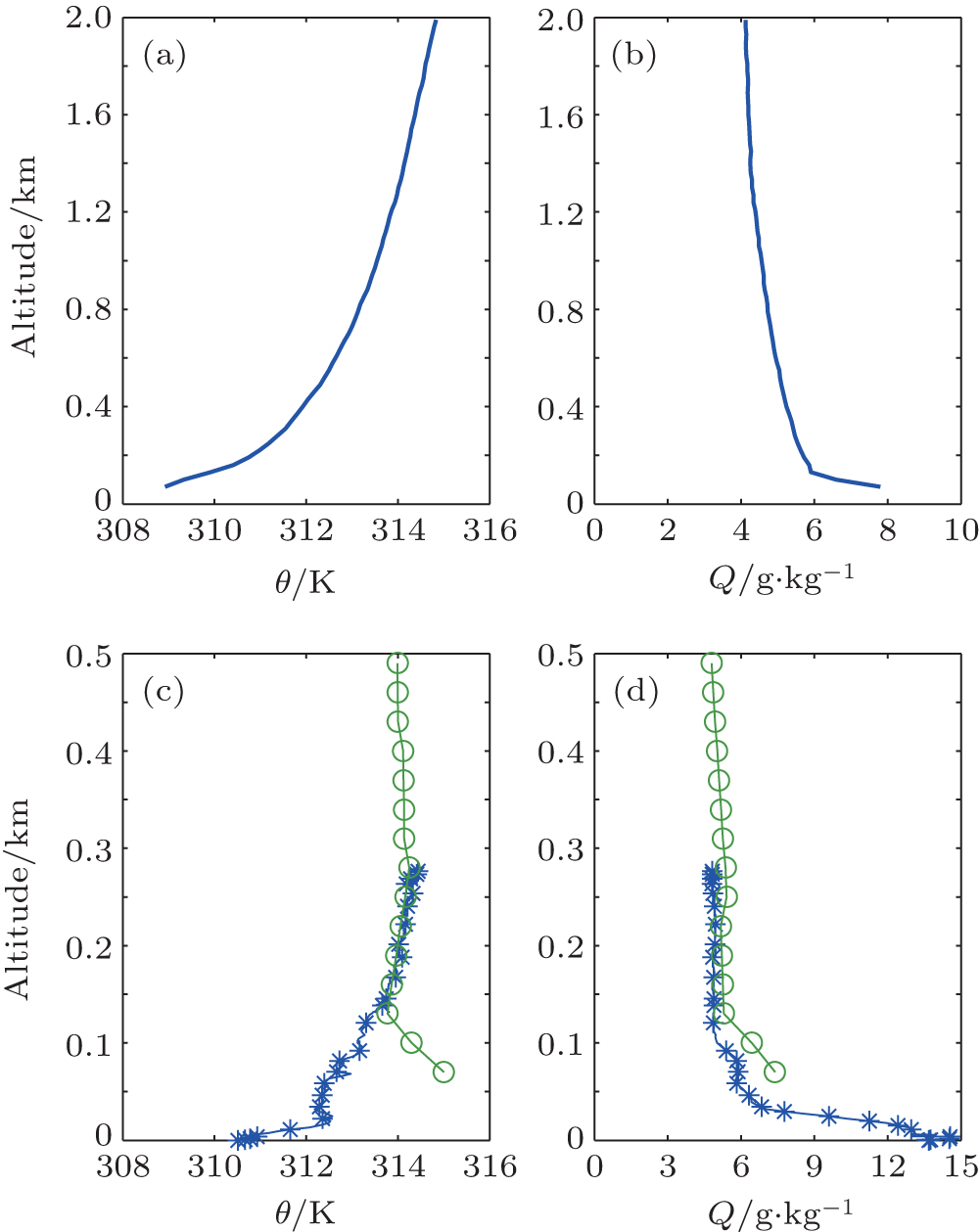
Conventionally, meteorological data, i.e., atmospheric pressure P, temperature T, and humidity RH, can be determined via radiosonde sounding measurement. In this work, a modern high resolution GPS radiosonde (Changfeng CF–06–A[26]) tied to a carrier of captive balloon was employed to measure meteorological parameters at different altitudes. Compared with classical ones, GPS radiosondes have higher vertical resolution (sampled at 1-s intervals) which would make the diagnosis of small scale duct structures possible.[17,26] The use of captive balloon can provide a much higher vertical resolution of less than 1 meter by controlling the carrier’s ascent rate manually, which outclasses the resolution of Vaisala RS products used in EU and India.[11,27] All the radiosondes were launched over a new littoral station (41.89° N, 87.22° E) on the south bank of the Lake, just near the bottle-neck between the main lake and the small adjacent lake in the southeast corner. In this paper, the maximum height to which the balloon went was limited to 500 m, which was high enough for us to detect almost all of the ducting events over the Lake. Since the specific humidity Q decreases sharply (the most important reason for which ducting events happen) within the first 200-m layer over the Bosten Lake Basin according to an analytical result of historical radiosonde data recorded at a classical radiosonde station which lies more than ten kilometers southeast of the littoral station, which is shown in Fig. 2. Figures 2(a) and 2(b) show the mean potential temperature θ and specific humidity Q in August, 2014. Although there exist some differences in θ-profiles and Q-profiles over the two stations (see Figs. 2(c) and 2(d)), fortunately, as shown in Figs. 2(c) and 2(d), the discrepancy is much larger just near the underlying surface, at an altitude higher than 150 m over the Lake, both the θ-profiles and Q-profiles tend to be equal, so an maximum detection height of 500 m is high enough. From Figs. 2(c) and 2(d) we can see that the discrepancy of θ-profiles over the two stations is much larger than that of Q-profiles, the main reason is that lake breeze dominates along the lakeshore before the sunset in a clear day and a temperature inversion is prevailing over the littoral station, but over the classical station far away from the Lake, the hot landmass heats the surface air continually, air temperature will decrease rapidly within the first 60-m layer which results in a drop of potential temperature near the surface.
Fig. 2. The mean (a) potential temperature θ and (b) specific humidity Q in August, 2014 over the classical radiosonde station. Typical profiles of (c) potential temperature θ and (d) specific humidity Q observed over the two stations on 11 August 2014 at 2000-h CST. Lines with circles represent the profiles observed over the classical radiosonde station, and lines with stars represent the profiles observed over the littoral station.
It should be emphasized that there is a discrepancy between the local time (LT) and China Standard Time (CST), that is LT = CST-0200 h, and the high noon at the local area is about 1400-h CST. As a general rule in China, CST will be used in this paper. On the basis of the weather conditions in a day over the Lake, days are divided into early morning (0800-h to 1000-h CST), forenoon (1000-h to 1400-h CST), and afternoon (1400-h to 2100-h CST, i.e., between the noon and sunset). The sounding experiments began on 15th July and finished at the end of August. Because of some technical reasons, only a few data were collected during July. All of the radiosondes were launched on clear days and majority of these radiosondes were launched during the forenoon with a time interval about one hour or two. Similar to Zhao Xiao-feng et al.,[17] we employed several data quality control methods to eliminate unreasonable measurements before taking statistics. Evident inaccurate datasets were eliminated at the first sight, and singular points, which were common for high-resolution GPS radiosonde measurements, were eliminated by a Kernel smoother. For points with a great difference between measurements and smoothing results were eliminated.
2.2. Identification of atmospheric ducts
During the two months, 102 datasets were obtained, six of which were invalid. For each dataset, M-profiles were calculated from temperature, pressure, humidity, and altitude via Eq. (1), and then duct altitude, corresponding strength, and its thickness were calculated from M-profiles. Following Basha G et al.,[11] we define the duct altitude as the altitude of the top of the trapping layer. The duct thickness refers to the difference between the base altitude and the duct altitude (see Fig. 1(c)). Yet, in this work, only an M-profile that has a negative gradient structure with a difference larger than 4.4 M-units, compared with the M-profile of standard atmosphere, can be identified as a duct. Since the measurement uncertainty of modified refractivity is about 4.4 M-units under a common condition over the Lake where T = 25 °C, P = 880 hPa, RH = 65%. Among the 96 valid sets of data, 78 (81%) ducting events were observed, more detailed results will be shown later.
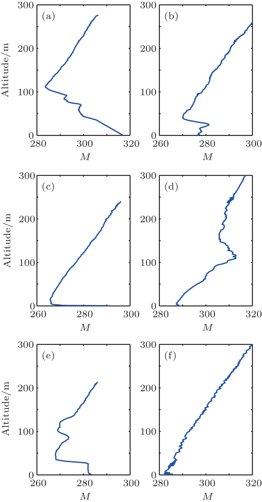
Fig. 3.M-profiles for several types of ducts observed over Bosten Lake in 2014: (a) surface duct observed on 26 July at 1140-h CST; (b) surface-based duct observed on 7 August at 1130-h CST; (c) evaporation duct observed on 28 August at 1230-h CST; (d) elevated duct observed on 22 August at 0830-h CST; (e) complex duct observed on 1 August at 1820-h CST; (f) standard atmosphere condition observed on 1 August at 1140-h CST.
Ducting occurs when the gradient of modified refractivity, i.e., dM/dz, turns negative. Fortunately, all the five types of ducts mentioned earlier were observed over the Lake, which are illustrated in Fig. 3. According to an analysis of the 78 observed ducting events and their corresponding M-profiles, surface ducts and surface-based ducts occurred frequently over the Lake in the daytime, figures 3(a) and 3(b) show the typical profiles of surface duct and surface-based duct observed over the Lake. The other three types of ducts were rarely observed. However, not all the observed surface and surface-based ducts have an idealized M-profile that listed in any textbook. Most generally, as illustrated in Fig. 3, small-scale variations along the profiles always occurred. The small-scale variations were omitted when the profiles were being normalized to idealized ones that shown in Fig. 1.
2.3. Diurnal variation of ducts
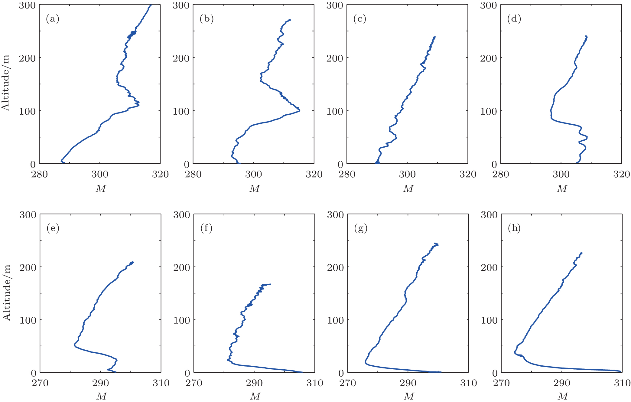
Ducting conditions are significantly influenced by the meteorological conditions. As for Bosten Lake, it experiences a strong diurnal variation in air temperature and humidity during the daytime; therefore there will be significant variations in the ducting occurrence, duct altitude, duct strength, and its thickness. Figure 4 presents a typical example of the diurnal ducting variations observed on 22 August 2014. The figures show that elevated ducts were observed (Figs. 4(a) and 4(b)) in the early morning, followed by standard atmosphere (Fig. 4(c)) and surfaced-based ducts (Figs. 4(d) and 4(e)), lastly surface ducts (Figs. 4(f)–4(h)) were observed in the afternoon. Additionally, in the early morning, the observed ducts have a higher altitude, but weaker strength; by contrast, the ducts observed after the noon have a lower altitude, but stronger strength. Moreover, the statistical result can be seen below.
Fig. 4. Ducting variations on 22 August 2014: (a) observed at 0830-h CST, (b) observed at 1030-h CST, (c) observed at 1130-h CST, (d) observed at 1220-h CST, (e) observed at 1410-h CST, (f) observed at 1610-h CST, (g) observed at 1820-h CST, (h) observed at 2000-h CST.
As mentioned earlier, 78 ducting events were observed within the 96 valid datasets obtained during the two-month experiments. Table 1 shows the daily distribution of ducting events along with the number of obtained datasets and their corresponding ducting occurrence in detail.
According to Table 1, we can see that the ducting occurrence probability in a clear day was at its minimum in the early morning, followed by forenoon, and then reached its maximum in the afternoon, that is between the noon and sunset. However, some occurrence probability data listed in the table are not so accurate because of the limited sampled data in early morning; a meteorological analysis result will draw the same conclusion later.
Table 1.
Table 1.
Table 1.
Distribution of ducting events during daytime along with number of datasets.
.
Parts of a day
Duct characteristics
Early morning
Forenoon
Afternoon
Ducting events/datasets
5/11
49/61
24/24
Ducting occurrence
45.5%
80.3%
100.0%
Table 1.
Distribution of ducting events during daytime along with number of datasets.
.
Besides the ducting occurrence, other duct characteristics, i.e., duct altitude, duct strength, and duct thickness, are very important while assessing the EMW propagation, for they determine the trapping capability of a duct. The mean duct altitude, duct thickness, duct strength, and their corresponding standard deviations in every part of a day during the two months are listed in Table 2. It must be noted that, for a complex duct, only the first ducting layer was taken into account.
Table 2.
Table 2.
Table 2.
Statistical results of duct characteristics during a day.
.
Parts of a day
Duct characteristics
Early morning
Forenoon
Afternoon
Duct altitude/m
142.9±79.9
59.2±32.1
43.7±22.8
Duct thickness/m
43.9±25.8
39.8±23.8
42.6±22.9
Duct strength/M-units
7.5±2.8
13.7±7.9
31.3±12.1
Table 2.
Statistical results of duct characteristics during a day.
.
From Table 2, it is observed that the mean duct altitude experienced a decrease in a clear day during the two months: the duct altitude was at its maximum in the early morning, and decreased in the forenoon, finally reached its minimum in the afternoon. Contrarily, the duct strength was at its minimum in the early morning, and then followed by the forenoon, finally it reached its maximum in the afternoon. We can also see from Table 2 that the discrepancy in values between the duct altitude and duct thickness before the noon (in the early morning and forenoon) was larger than that in the afternoon, this implies that elevated duct and surface-based duct were prevailing before the noon, but surface duct dominated after the noon (see Fig. 4), because the duct thickness was the same as duct altitude in a surface duct. Additionally, the maximum duct altitude observed was about 269 m, which was observed on 22 August 2014 at 0930-h CST (due to the limited space, it was not listed in Fig. 4), and its corresponding strength and thickness was about 8.1 M–units and 80.6 m respectively. The maximum duct thickness observed was about 112 m, which was observed on 26 July 2014 at 1140-h CST (surface duct, Fig. 3(a)), and its corresponding strength was about 33.3 M–units. The strongest duct strength observed was about 53.1 M–units, which was observed on 12 August 2014 at 2040-h CST (surface duct), and its corresponding thickness was about 11.1 m.
Briefly, the ducting conditions experienced a strong diurnal variation in a clear day during the two months. In a clear day, the ducting occurrence increases from early morning to forenoon, and then reaches nearly 100% in the afternoon. Similarly, the duct strength increases from early morning to forenoon, and then reaches its maximum in the afternoon. Higher altitude duct (as well as thicker duct) is observed in the early morning when elevated ducts may occur, then followed by forenoon, and becomes lower in the afternoon when surface ducts prevail.
3. Meteorological reasons for diurnal ducting variation
In the preceding section strong diurnal variations in ducting condition are noticed in clear days. The main reason for the strong diurnal variations is large diurnal changes in air conditions, i.e., potential temperature and specific humidity over the Lake.
In a calm, early morning of a clear day in the two hottest months (July and August) in Bosten Lake Basin, just during the two more hours after the sunrise, temperature inversion resulting from radiative cooling of the surface still keeps alive with an altitude of several hundred meters, which is favorable for the formation of a stable boundary layer (SBL). Since the surface is emitting more radiation energy than it is receiving from solar radiation during that time. The strong stability in an SBL will suppress the vertical convection of water vapor, so the specific humidity in a radiation inversion layer will vary slowly with height generally, a sharp decrease at high altitudes is unusual, but as shown earlier, elevated duct might happen in the early morning. As an accepted scenario, the main reason for the formation of elevated ducts is subsidence motion[4,5,11,16] which can last for several days, but some observed elevated-duct cases did not predict subsidence motion, such as the elevated duct observed on 22 August 2014, and why this happened? Stull R B[28] and Ohya Y et al.[29] indicated that occasional bursting of turbulence could be found in a SBL with strong stability, and a turbulent bursting would cause sporadic vertical mixing. If a bursting event occurs on the ground or lake surface, it will bring an abundance of water vapor upward at a high altitude over the Lake due to buoyancy, and the temperature inversion will prevent it from diffusing into a higher layer above the inversion layer. When water vapor associated with turbulence bursting advect over the Lake, an elevated duct will occur. Sun J L et al.[30] have once observed that a solitary wave with high specific humidity was propagating in a nocturnal SBL at Leon, Kansas, USA in October 1999. The elevated duct observed in the early morning of 22 August has certainly resulted from turbulent bursting, for an obvious potential temperature inversion (the so called overturn) was observed at a depth of about 150 m (see Fig. 5(a)).
Contrary to temperature inversion, a potential temperature inversion is defined as a localized decrease of potential temperature versus height, which is generated by turbulence or Kelvin–Helmholtz billows.[31] As illustrated in Fig. 5(b), high specific humidity was observed in the range of 60 m–150 m deep where was the duct structure located, which suggest that the turbulence might be initiated at the ground and propagated upward to about 150 m since the water vapor concentrations normally decreases with the altitude in a thick SBL. Because the subsidence motion and turbulent bursting do not frequently occur in the two months, and the stability in a thick SBL will suppress the convection of water vapor, the Lake experiences a lower ducting occurrence and weaker strength in the early morning.
Fig. 5. Typical profiles of potential temperature θ and specific humidity Q observed on 22 August 2014: (a) potential temperature and (b) specific humidity profiles observed at 0830-h CST; (c) potential temperature and (d) specific humidity profiles observed at 1220-h CST; (e) potential temperature and (f) specific humidity profiles observed at 1410-h CST; (g) potential temperature and (h) specific humidity profiles observed at 2000-h CST.
As time passes, the surface receives more energy from solar radiation than emitting radiation, then the surface heats the air continually, at last, the inversion will be eliminated in the mid-morning, air temperature will decrease linearly near the surface, so does the specific humidity, as a result, standard atmosphere will be observed, which is shown in Fig. 4(c). From then on, transpiration and evaporation over the land near the Lake becomes stronger, the atmosphere is dominated by vertical air motion, and enormous water vapor is erupted into the surface layer. To a lesser extent, both of the potential temperature and specific humidity have a uniform distribution in the mixed layer,[28] which is illustrated in Figs. 5(c) and 5(d), as a result, surface-based duct will be observed, just as shown in Fig. 4(d).
After the noon, lake-breeze prevails along the lakeshore line, and becomes stronger and stronger as time passes in the afternoon, which is the main reason for the ducting formation during that time. Cool air from the Lake moves across the warm land near the lakeshore line with a velocity of several meters per second, a return circulation (the anti-lake-breeze) aloft brings the warmer, low-humidity air back to the middle of the Lake where it descends toward the Lake surface to close the circulation,[28,32,33] as a result, a temperature inversion with a depth less than 100 m and an increase in humidity over the warm land near the lakeshore line will be formed, which is depicted in Figs. 5(e) and 5(f). This is known as capping inversion, which will “shut off” almost all the convection and result in a sharp decrease in specific humidity (Fig. 5(f)). Consequently, a stronger surface or surface-based duct happens (see Figs. 4(e)–4(g)). In the later afternoon, just near the sunset, the land surface temperature reaches its maximum during a day, then will decrease as time goes on, for the surface emits more radiation energy than receives from solar radiation because of the lower sun angle at that time, lake-breeze also becomes weaker, too. As a result, a thinner surface temperature inversion will be observed (Fig. 5(g)). Because of the large heat capacity of the Lake, evaporation will continue, and enormous water vapor will advect over the land, simultaneously, the very thin surface temperature inversion will suppress the convection of water vapor which will prevent it to diffuse into a higher layer and result in a sharp decrease in specific humidity (Fig. 5(h)). As a result, the strongest surface duct will be observed in the later afternoon (Fig. 4(h)). Briefly, lake-breeze circulation is the most prevalent phenomenon between the noon and evening in a clear day around a lake, so the ducting occurrence is very high during that time.
4. Ray-tracing framework for EMW propagation
To assess the performance of radar or HPM in a ducting environment, an EMW propagation model must be provided. Although parabolic wave equation method are widely used to model the field distribution of EMW, ray-tracing can provide a rather intuitive tool for modeling the propagation characteristics, such as propagation paths, critical angle, shadow zone, refraction angle, grazing angle, and etc.,[34,35] which is also widely used in recent years, too.[2,35] However, most of the previous methods for ray-tracing were based on small angle approximation, here we will present a ray-tracing technique based on Runge–Kutta method.
4.1. Ray-tracing equation
Consider a ray passes through a stratified atmosphere above a spherical Earth where refractive index n depends on the height above the Earth’s surface H only, the path of a radio wave will obey the Snell’s law
where α is the local elevation angle of the ray; r = ae + H where ae is the local earth’s effective radius; ϕ is the polar angle. We use the conformal transformation provided by Levy M[25] to convert the spherical coordinate system to a plane one, which is given by
After the transformation, the Snell’s law becomes
where m is the modified refractive index, i.e., m = n + z/ae. Since z is very small compared to the Earth’s radius ae, the exponent term in Eq. (4) can be approximated by the Taylor method. Then a nonlinear differential equation (DE) can be obtained by using the derivative of Eq. (4) with respect to x
where the prime denotes differentiation with respect to x. This equation is the so-called ray-tracing equation. In conjunction with the proper boundary conditions, equation (5) can be solved using Runge–Kutta algorithm, which can provide a stable and fourth-order accurate method. As for a second order DE like Eq. (5), it can be changed into a system of DEs of first order
where z1 represents the variable z, and z2 represents z′ respectively. Suppose the value of the numerical solution at the point x = xj is denoted by (xj, z1j, z2j), choose a step size h, the Runge–Kutta formula is given by[36]
where the subscript i represents 1 and 2. Additionally, the path length (range) at the interval [xj, xj + h] can be calculated using trapezoidal numerical integration method.
which can avoid the singular point of the traditional path length integral for radar measurement, but is equivalent to the traditional one. When a ray reaches the surface, it will be reflected, and then the step size h should be updated. That is if z1j > T(xj) but z1, j+1 < T(xj + h), where T(x) is terrain height at x, the solution (xj+1, z1,j + 1, z2,j + 1) will be eliminated, and replaced by a new point where the new step size hN should be selected to make meet the terrain surface. A robust iteration method, such as bisection method,[36] is used to solve hN. When a ray is incident on an irregular terrain with a slope angle of β, z2 should be replaced by the slope of the reflected ray K
where K0 is the slope of the incident ray, i.e., that mentioned earlier.
4.2. EMW propagation characteristics
Furthermore, equation (5) can be partially solved to a nonlinear DE of lower order
where p is the first derivative of z, i.e., p = dz/dx; C is a constant determined by the initial conditions. It is apparent that the critical angle can be calculated precisely from Eq. (10). Critical angle θc denotes the corresponding launching angle when the ray travels horizontally at the duct top, so
where m0 and mu denote the modified refractive index at the height of the transmitting antenna and that at the top of the ducting layer, respectively. Eq. (11) implies that only the rays launched by a source located in the ducting layer at an angle α less than the critical angle (|α| < θc) can be trapped in the duct. If the source is located above the ducting layer with a launching angle α within the interval [–θc, 0), the rays will be totally reflected, no signal can reach the ducting layer and below. In a similar way, the grazing angle θg, i.e., the complement of the incident angle, can be calculated precisely, too
where ms denotes the modified refractive index at the surface; β is the slope angle of the terrain; α0 is the initial launching angle.
Additionally, assume that the target is located at (xT, zT) in the new coordinate, the refractive errors of the range ΔR and height ΔH for radar measurement can be calculated,
where H0 is the height of the transmitting antenna; R is the measured range by a radar.
4.3. Numerical experiments
To visualize the ducting effect on the radar or HPM performance, here we will show some simulation results about EWM propagation in the ducting environments observed over the Lake (shown in Fig. 3) using the ray-tracing technique presented earlier. As for an arbitrary M-profile, the partial derivative of m with respect to variable z can be calculated by using numerical difference method. However, in this paper, all the observed elevated duct, surface duct and surface-based duct were normalized to tri-linear profiles, and the observed evaporation duct was also normalized to a standard one, which made us to calculate the partial derivative of m more easily.
Table 3.
Table 3.
Table 3.
Parameters in the simulation and the corresponding ducing characteristics.
.
Duct type
Parameters
SurDa
SurbDb
EvaDc
EleDd
Antenna height/m
5
5
3.5
100
Beam-width/(°)
2
2
2
2
Elevation angle/(°)
0.5
0.5
0.5
-0.5
Duct altitude/m
111
40.4
14
169.1
Duct thickness/m
111
40.4
14
86.2
Duct strength/M-units
33.3
11.4
24.6
8.0
Surface duct
Surface-based duct
Evaporation duct
Elevated duct.
Table 3.
Parameters in the simulation and the corresponding ducing characteristics.
.
Figure 6 shows the ray-tracing result of EMW paths through several ducting environments, which were listed in Fig. 3, with a launching angle step of 0.02°. Moreover, other simulation parameters for the antenna and the corresponding ducting characteristics were listed in Table 3.
As for the simulations illustrated in Fig. 6, the last two cases use the same antenna parameters as the first one does, and the last case use the same M-profile as the second one does. Compared with the standard atmosphere condition in Fig. 6(e), the radar beams can be partially trapped in the ducting layers (Figs. 6(a)–6(d)) when propagated in a ducting environment, which will “split” a beam into two parts. Certainly, only when the transmitter is located in the ducting layer and its launching angle less than the corresponding critical angle can ray trapping happen. According to Eq. (11), we can calculated the corresponding critical angles for the four simulation cases (Figs. 6(a)–6(d)), which are 0.4569°, 0.2274°, 0.0991°, and 0.1529° respectively. From this we can see the trapping ability of each duct apparently. The maximum grazing angles of the trapped rays for the first three cases (Figs. 6(a)–6(c)) are 0.4675°, 0.2144°, and 0.4015° respectively. For case 4 (Fig. 6(d)), the trapped rays cannot reach the surface, but we can calculated the grazing angle of the boresight which is 0.3360°. From the first four simulation cases shown in Fig. 6, we can see that there are some areas in the x–z plane (the right panels in Figs. 6(a)–6(d)) above or below the ducting layer that it has no rays there, which indicates a very low ray density and very weak field strength there; they are the so-called shadow zones or radar holes. Moreover, we can see that it has a higher ray density in some areas in the x–z plane, which means a stronger intensity of electromagnetic field there. Figure 6(f) shows that when the trapped ray paths meet an irregular terrain, they will be reflected, and most of them will not be tapped again. According to the simulation, we can get some refractive errors of radar measurements. Here, we will show some refractive errors of radar measurement in the surface duct listed in Table 3 (case one of Fig. 6), just as shown in Table 4. In this table, it is shown that as the total range increases, both the range and height errors increase. Compared with the height error, the range error is much smaller. If a ray is tapped (elevation angle is less than the critical angle) in the ducting layer, the height error is much larger than the condition that no trapping happens when the total range is longer than 60 km.
Fig. 6. EWM propagation in different environments: ray-tracing paths in (a) surface ducting environment, (b) surface-based ducting environment, (c) evaporation ducting environment, (d) elevated ducting environment, (e) standard atmosphere environment, and (f) surface-based ducting environment over irregular terrains. The left panels show the corresponding M-profiles normalized from Fig. 3.
The ray tracing method present in this work is a convenient tool to assess the performance of radar, HPM or communication systems in a ducting environment which can provide a rather intuitive picture for EMW propagation, as well as some precise propagation characteristics. In addition, we compared the square of the first derivative of z (i.e., p2 in Eq. (10)) with the analytical solution shown in Eq. (10). The result has shown that the relative error was less than ten-millionth percent for most of the cases, only when the absolute value of p became less than 1.0 × 10⁻⁴ did the relative error turn to about ten thousandth percent. That means the method can provide a very high accuracy for ray paths.
Table 4.
Table 4.
Table 4.
Range/height errors of radar measurement in a surface duct. The values in the bracket represent the refractive height errors of radar measurement.
.
Elevation angle/(°)
Total range/km
0.10
0.25
0.40
0.60
40
12.7(190.6)
12.5(273.5)
12.1(365.4)
10.9(200.4)
60
19.1(385.8)
18.9(542.5)
18.5(639.1)
16.1(332.9)
80
25.7(645.9)
25.3(820.7)
24.5(990.8)
21.1(476.1)
100
32.5(956.7)
32.1(1200.0)
31.7(1456.9)
25.9(630.0)
Table 4.
Range/height errors of radar measurement in a surface duct. The values in the bracket represent the refractive height errors of radar measurement.
.
5. Conclusion
The effect of the atmospheric ducts upon EMW propagation is important for many radio systems. In this paper we present a two-month (in July and August, 2014) observation of the atmospheric ducts over Bosten Lake using high resolution GPS radiosonde for the first time. Strong diurnal variation in ducting characteristics is noticed in a clear day and the features of the ducting environments are discussed in detail. Ducting occurrence increases from early morning to forenoon, and then reaches its maximum (nearly 100%) in the afternoon. So does the duct strength. But contrarily, duct altitude experiences a decrease in a clear day. The main reason for the diurnal ducting variation is as follows:
In the early morning, radiative inversions do exist, thicker SBL will suppress the convection of water vapor, a possible reason for duct formation is turbulent bursting which means a lower ducting occurrence and weaker duct strength, and elevated duct may occur at that time, which means that higher altitude duct and thicker duct will be observed.
During forenoon, evaporation becomes stronger, vertical air motion dominates in the surface layer, then the ducting occurrence and duct strength will increase, duct altitude and thickness will decrease.
After the noon, lake-breeze prevails over the lakeshore, thinner and stronger front inversion layer will last for several hours, thus, the ducting occurrence and duct strength reaches their maximum in a day. Surface duct dominates during that time, which means a lower duct altitude and thinner duct thickness.
A novel ray-tracing framework based on Runge–Kutta method is present to assess the performance of radio systems in a ducting environment, and precise critical angle and grazing angle for a duct derived from the ray-tracing equations are provided. The range/height errors for radar measurement induced by refraction has also been presented, too. Numerical experiments on EMW propagation in the observed ducting environments with the ray-tracing framework have been carried out with high accuracy. The results of the numerical investigations have demonstrated the significant influence on radio systems of atmospheric ducts, for example ray trapping, beam splitting, detecting shadow, refractive errors, and so on.
This study will also serve as a complementary study of atmospheric duct for the endorheic lakes in Xinjiang Uygur Autonomous Region. In future studies, ducting conditions in other seasons would be investigated, and new technique for determining ducts can be used.
Reference
1
SkolnikM I2001Introduction to Radar System3rd edn.SingaporeThe McGraw-Hill Companies, Inc.502518
EssenHFuchsH HPagelsA2006Proceedings of SPIE 6364, Optics in Atmospheric Propagation and Adaptive Systems IXSeptember 11–13, 2006Stochholm, Sweden63640810.1117/12.693498
8
WillisM JCraigK H2007Proceedings of the 2nd European Conference on Antennas and PropagationNovember 11–16, 2007Edingburgh, UK138


 , Ning Hui, Tang Jing, Xie Yong-Jie, Shi Peng-Fei, Wang Jian-Hua, Wang Ke]