

Simulation of the 3D viscoelastic free surface flow by a parallel corrected particle scheme
[Ren Jin-Lian†,  , Jiang Tao]
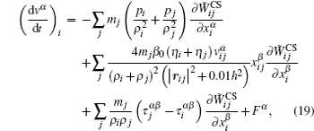
, Jiang Tao]
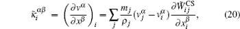
|
|


† Corresponding author. E-mail:
Project supported by the Natural Science Foundation of Jiangsu Province, China (Grant Nos. BK20130436 and BK20150436) and the Natural Science Foundation of the Higher Education Institutions of Jiangsu Province, China (Grant No. 15KJB110025).
In this work, the behavior of the three-dimensional (3D) jet coiling based on the viscoelastic Oldroyd-B model is investigated by a corrected particle scheme, which is named the smoothed particle hydrodynamics with corrected symmetric kernel gradient and shifting particle technique (SPH_CS_SP) method. The accuracy and stability of SPH_CS_SP method is first tested by solving Poiseuille flow and Taylor–Green flow. Then the capacity for the SPH_CS_SP method to solve the viscoelastic fluid is verified by the polymer flow through a periodic array of cylinders. Moreover, the convergence of the SPH_CS_SP method is also investigated. Finally, the proposed method is further applied to the 3D viscoelastic jet coiling problem, and the influences of macroscopic parameters on the jet coiling are discussed. The numerical results show that the SPH_CS_SP method has higher accuracy and better stability than the traditional SPH method and other corrected SPH method, and can improve the tensile instability.
The complex jet coiling phenomena,[1] although they play an important role in many industrial processes, such as extrusion, and container filling with polymers, are still less well understood in terms of fundamental fluid dynamics. In order to predict the complex rheological phenomena in a real three-dimensional (3D) viscoelastic jet buckling process, a number of grid-based numerical methods have been proposed, such as the finite difference method (FDM), finite element method (FEM), finite volume method (FVM), etc. The mesh-based methods mentioned above have been applied to many fluid mechanic fields.
However, these grid-based methods also suffer numerical difficulties, such as severe mesh distortion, and the expensive cost in the mesh generation process. As one may expect, the various mesh-free methods[2–4] in a Lagrangian framework have been proposed to solve the fluid dynamic problems, such as the smoothed particle hydrodynamics (SPH) method,[4,5] element-free Galerkin (EFG) method,[3] reproducing kernel particle method (RKPM),[6–8] and so on.
The SPH method[5] is a pure meshless method which employs Lagrangian description of motion. Recently, the SPH method has been extensively applied to the fluid dynamic areas due to its merits, such as viscous flows,[9] free surface flows,[5,10,11] incompressible fluids,[12,13] multi-phase flows,[14] and non-Newtonian fluid flows.[13,15] However, the application of the SPH method to the viscoelastic fluid mainly focuses on the two-dimensional (2D) viscoelastic jet buckling, and the application of the SPH method to the 3D viscoelastic jet coiling has received a little attention recently. The reason is that the SPH method usually suffers two major drawbacks, that is, the particle inconsistency[16,17] for uninformed particle distributions/near the boundary domain and the numerical/tensile instability.[18] In order to restore the consistency of the kernel and gradient particle approximations of SPH, some improved SPH methods based on the Taylor series expansion have been proposed, such as the corrected smoothed particle hydrodynamics method (CSPM),[19] finite particle method (FPM),[11,20] the modified SPH (MSPH) method,[21] and the symmetric SPH (SSPH) method.[22] Although these improved methods have higher accuracy than the traditional SPH (TSPH) method, some disadvantages still exist and make it more difficult to be extended to the complex fluid dynamic problems,[22] the choice of the kernel function is limited for solving the partial differential equations (PDEs) with higher derivatives; the local matrix is asymmetric, which can cause numerical instability; its computational efficiency is lower than that of TSPH, such as the MSPH method and SSPH method. Therefore, a corrected kernel gradient scheme[23] has been introduced into the TSPH method and extensively applied to Newtonian fluid[24,25] in recent years. However, the corrected kernel gradient scheme has been rarely extended to simulate the viscoelastic jet buckling, especially the 3D simulations of the viscoelastic jet coiling.
In the present paper, the 3D viscoelastic jet coiling process based on the Oldroyd-B model is simulated and analyzed by a parallel coupled corrected particle scheme named the SPH_CS_SP (SPH with a corrected symmetric kernel gradient scheme and shifting particle technique) method. Some special phenomena of the 3D jet coiling are observed and the physical explanations of these complex phenomena are also analyzed. The proposed particle method combines three improved concepts, that is, introducing the incompressible condition in the momentum equation to achieve better robustness,[26] extending the corrected symmetric kernel gradient scheme[27] to further improve the numerical accuracy and employing the shifting particle technique to overcome the tensile instability.[28] It should be noted that the main difference between the proposed SPH_CS_SP method and other improved SPH methods lies in the following respects: (i) the obtained discretized form of momentum equation is different from those in Refs. [24] and [25]; (ii) the shifting particle technique is first applied to the viscoelastic fluid flows; (iii) the presented corrected SPH method is different from the particle methods in Refs. [24] and [29], which have not been extended to simulate the 3D polymer free surface flow.
The rest of this paper is organized as follows. The governing equations and the viscoelastic constitutive model are introduced in Section 2. In Section 3, the details of the proposed SPH_CS_SP scheme for the viscoelastic fluid are described. The accuracy and robustness of SPH_CS are tested by simulating the Poiseuille flow in Section 4. Moreover, the necessity of enforcing the shifting particles technique is also investigated by simulating the Taylor–Green flow in Section 4. In Section 5, the capacity for SPH_CS_SP to simulate the viscoelastic flow is verified by the polymer flow around a periodic array of cylinders. In Section 6, the proposed particle method with MPI parallelization technique is extended to simulate the 3D viscoelastic jet coiling problem in the filling process. Some conclusions are drawn from the present study in Section 7.
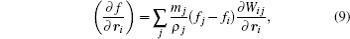
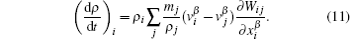
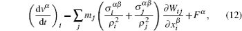
In the 3D Lagrangian frame, the governing equations of a weakly compressible fluid can be described as follows:


In this paper, we choose the Oldroyd-B model as the constitutive equation, which represents the basic viscoelastic fluid and shows complex rheological behavior of polymer flow. The extra stress tensor


Moreover, some parameters are introduced, that is, the total viscosity η = ηs + ηp, the ratio of Newtonian and polymeric viscosity β0 = ηs/(ηs + ηp), the Reynolds number Re = (ρUL)/η, and the Weissenberg number We = (λ0bU)/L, where U and L represent the characteristic velocity and length, respectively.
Like many previous studies,[4,9] here we also treat the incompressible flows as a slightly compressible fluid by a suitable equation of state, that is[10]

In order to accurately simulate the viscoelastic fluid flow, a new corrected particle scheme is proposed. It mainly combines three different improvements, that is, introducing the incompressible condition in the momentum equation to achieve better robustness,[26] applying the corrected symmetric kernel gradient method[29] to the discrete form of the first derivative to improve the numerical accuracy, and employing the shifting particle technique to overcome the tensile instability.[25,26,28]
As is well known, in the traditional SPH method, the particle approximation for a function f and its first derivative at particle i can be written as[4,5]

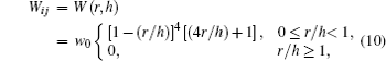
The kernel function is related not only to the accuracy but also to the efficiency and the stability of the resulting algorithm. As shown in Ref. [29], the Wendland function can produce more accurate results than the common spline kernel functions. So the following quintic Wendland kernel function is adopted:
According to Eq. (
Considering the discrete gradient scheme


The particle discretized scheme of total stress equation (

The TSPH discretized formulas (
Firstly, introducing the incompressible condition into momentum equation (

Secondly, the corrected symmetric kernel gradient scheme[27] and the Taylor expansion concept[18] are also applied to the first-order derivative and the elastic stress part of Eq. (
It should be noted that the discretized form Eq. (
At the end of each time-step, the position of each particle is updated by

Finally, a shifting particle technique,[28] which is applied only to the viscous fluid now, is extended to the viscoelastic fluid to obtain a uniform particle distribution and further improve the tensile instability. Next, we describe the shifting particle technique in detail.
After each time-step, the position of particle i is shifted according to the following formula:


For simplicity, the method that combines the three different improvements is named the SPH_CS_SP method.
In the SPH simulations, the boundary treatment is an important problem. Next, we will describe the boundary treatment used in this paper.
For the solid boundary, the approach of two types of virtual particles[27] is extended to simulating the viscoelastic fluid flows in this paper. The first type of particle is placed on the solid wall, namely “wall particle”. The pressure and the components of the velocity of the wall particle i are calculated according to the following formula:

The second type of particle, called “dummy particle”, is placed just outside the solid wall, in a way which is similar to how the wall particle is located. In general, three layers of dummy particles are chosen. The pressure, velocity and extra stress tensor on the dummy particles are computed by the following formula:

In order to solve the system of ordinary differential equations (


As is well known, the time-step and space-step must satisfy the well-known Courant–Friedrichs–Lewy (CFL) condition for ensuring the numerical stability. According to Refs. [14] and [30], we may choose the following stability condition:
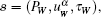
In this section, the Poiseuille flow of Oldroyd-B fluid is simulated by SPH_CS_CP method to test the capacity for the proposed SPH_CS method to solve the transient viscoelastic fluid, and the numerical results are compared with those obtained by TSPH method and the analytical solutions. It should be noted that the tensile instability does not exist in the simulations of the Poiseuille flow, and the shifting particle technique is not considered in this subsection.
Figure 
 | Fig. 1. Results for the Oldroyd-B fluid at different times with Re ≈ 0.03: (a) u(y); (b) τxy(y). |
Table

From Fig.
| Table 1. Relative L1-error norm of the velocity profiles for the case of Fig. |
Figure
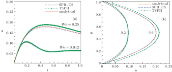
 | Fig. 2. Velocity profiles for the Poiseuille flow of Oldroyd-B fluid with different values of We and Re: (a) Re ≈ 0.03, u(y = 0.5); (b) Re = 1, u(y). |
The numerical results in Figs.
In this subsection, the 2D Taylor–Green flow[28] of the Newtonian fluid is simulated to show the necessity of the shifting particle technique.
The Taylor–Green flow is a periodic array of decaying vortices in the plane, and its velocity components are given
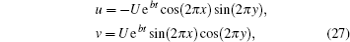
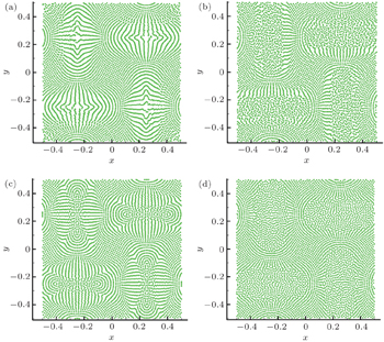
Figure
 | Fig. 3. Particle distributions obtained using different numerical methods with Re = 100, t = 0.2 s: (a) TSPH with cubic spline kernel; (b) TSPH with quintic Wendland kernel; (c) SPH_CS with quintic Wendland kernel; (d) SPH_CS_SP with quintic Wendland kernel. |
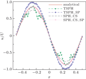
Figure
 | Fig. 4. Velocity profiles at x/L = 0.0 m with Re = 100, t = 0.2 s |
The numerical results show that the proposed SPH_CS_SP method indeed has higher accuracy and better stability than the TSPH, TSPH_SP and SPH_CS method, and it is necessary to combine the shifting particles technique with the corrected symmetric kernel gradient scheme.
The polymer fluid flow around a periodic array of cylinders[30–32] is usually regarded as a challenging test for the particle method. Here, we use it to test the reliability of the proposed SPH_CS_SP method to simulate the viscoelastic fluid.
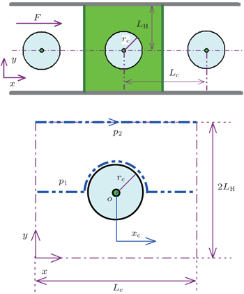
Figure 
 | Fig. 5. Geometric configuration of flow past a periodic array of cylinders: (a) periodic array of cylinders; (b) analog configuration of a single cylinder. |
In order to test the reliability of the SPH_CS_SP method of simulating the flow past cylinders, the same example of Newtonian fluid as that in Ref. [9] is first simulated by the SPH_CS_SP method. All the physical parameters are the same as those in Ref. [9], i.e., LH = 0.05 m, rc = 0.02 m, F = 5 × 10⁻⁵ m·s−2, ρ = 103 kg·m−3, η = 0.1 Pa·s, U = 1.5 × 10⁻⁴ m·s−1, c = 0.01 m·s−1, and Re = 0.03; the fluid particles are uniformly distributed in the whole domain, and the particle number Ny = 81 along the y axis. The time step Δt = 5 × 10⁻³ s, smoothing length h = 2.7d0.
Figure
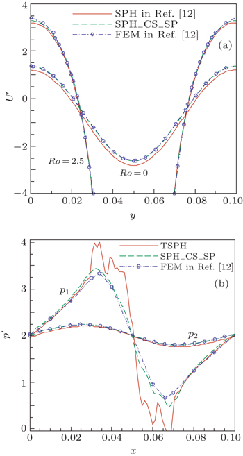
 | Fig. 6. Numerical results for the flow at stable state along different paths: (a) U; (b) pressure. |
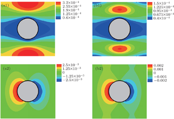
Figure
 | Fig. 7. Contour distributions of velocity U [(a1) and (b1)] and pressure [(a2) and (b2)] with different boundary conditions: (a1) and (a2) without confining a channel; (b1) and (b2) confined in a channel. |
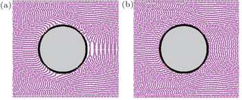
In order to demonstrate the capacity of the SPH_CS_SP approach for simulating the viscoelastic flow past a periodic array of cylinders, the Oldroyd-B fluid flow past a periodic array of cylinders is simulated and the particle distribution at stable state is shown in Fig.
Moreover, the following drag[32] for the viscoelastic fluid flow past a cylinder is introduced, which is
It can be seen that the so-called tensile instability appears near the cylinder in the SPH results (Fig.
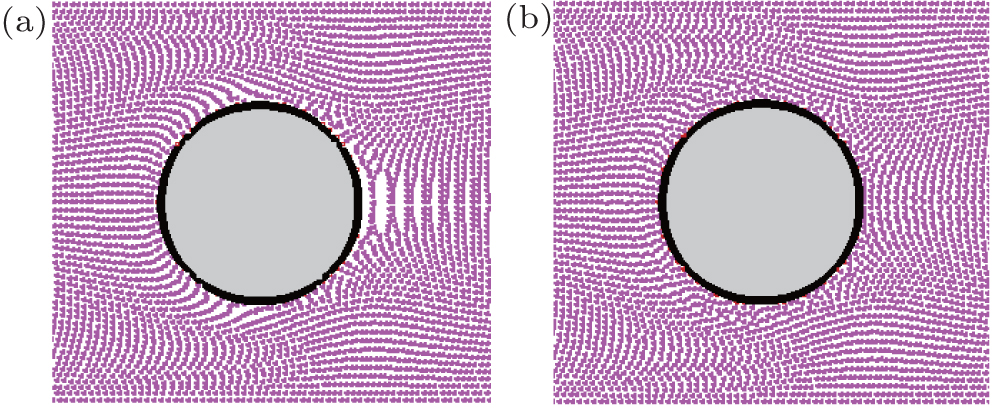 | Fig. 8. Particle distributions at stable state for Oldroyd-B fluid flow past a periodic array of cylinders with Lr = 6, We = 0.9: (a) SPH in Ref. [22]; (b) SPH_CS_SP. |
From Figs.
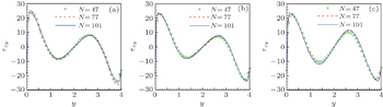
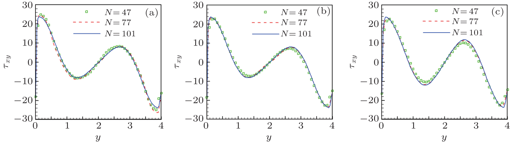
According to Ref. [17], the numerical convergence of SPH scheme not only depends on the particle numbers, but also relies on the smoothing length. Next, the simple numerical convergence is investigated by increasing the particle number Ny with different values of smoothing length h.
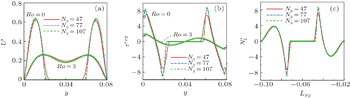
Figure 
 | Fig. 9. Curves of velocity (a), shear elastic stress (b), and first normal stress difference (c) along different paths with increasing the particle number at Lr = 6 and We = 0.06. |
Figure
 | Fig. 10. Shear elastic stresses along the path Ro = 2 with different values of smoothing length h (Lr = 6, We = 0.8, β0 = 0.2): (a) h = 2.0d0; (b) h = 2.4d0; (c) h = 2.8d0. |
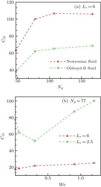
Figures
 | Fig. 11. Variations of drag coefficient with (a) Ny and (b) We. |
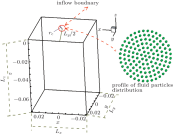
In order to demonstrate the ability of the proposed particle method to capture the complex free surface in the true flow, the 3D viscoelastic jet bulking problem of filling process in a rectangle container is simulated by the SPH_CS_SP method with the MPI parallelization technique. In this section, the instability phenomenon of jet coiling based on the Oldroyd-B fluid is mainly simulated and predicted.
The geometry of 3D jet bulking is shown in Fig.
 | Fig. 12. Sketch of 3D jet bulking. |
Figure
According to previous research,[34,35] the phenomenon of jet coiling based on the Newtonian fluid will occur, if Re < 0.5 and Lz/D > 10 or Re < 1.2 and Lz/D > 7 are satisfied. From Fig.
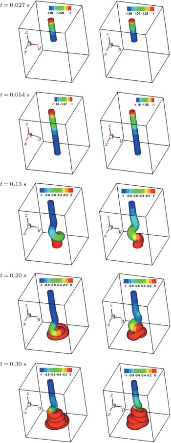
 | Fig. 13. The flow and w-velocity contours of the jet bulking based on the Newtonian (first column) and Oldroyd-B (second column) fluid with Re = 0.25 and We = 1. |
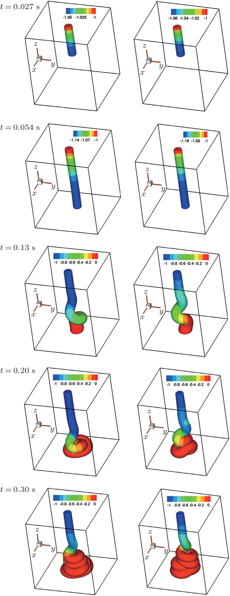
In order to clearly show the instability phenomenon of jet coiling, figure
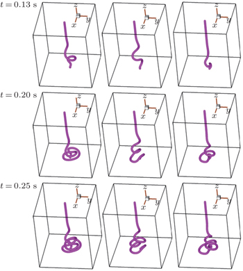
 | Fig. 14. Deformation processes of the center line of jet with Re = 0.25: Newtonian fluid (first column); Oldroyd-B fluid with We = 1 (second column), and We = 100 (third column). |
Next, the influences of macroscopic rheological parameters on the fluid deformation of filling process are predicted and discussed to further illustrate the complex phenomenon in the 3D viscoelastic filling process.
Observing Fig.
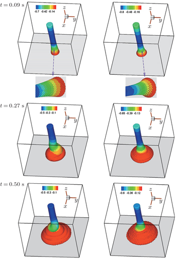
To further demonstrate the influence of We on the deformation process of jet coiling, we investigate the fluid deformations and the jet lengths of the jet buckling for the Oldroyd–B fluid with different Weissenberg numbers at Re=0.6. Here the jet length is defined as the distance from the jet front to the nozzle. The employed parameters are as follows: D = 6 mm, Lx = Ly = 6 cm, Lz = 5 cm (Lz/D = 8.3), U = −0.5 m·s−1, Δt = 5 × 10⁻⁶ s, υ0 = η/ρ0 = 0.005 m2·s−1 (Re = 0.6), λ0b = 0.006 s (We = 1), λ0b = 0.03s (We = 5), λ0b = 0.6s (We = 100), and the other parameters are the same as those in Fig.
 | Fig. 15. Filling deformation processes based on the Oldroyd-B fluid with Re = 0.6, We = 1 (first column) and 100 (second column) at different times. |
From Fig.
Figure
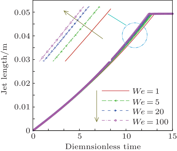 | Fig. 16. Variations of jet length of jet bulking with time for different values of We. |
Another macroscopic parameter which has an important influence on the deformation of jet fluid is the Reynolds number. Comparing Fig.
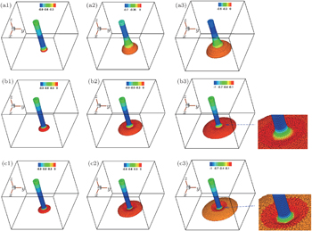
In order to further show the effect of the Reynolds number on the viscoelastic flow, figure
 | Fig. 17. Deformation processes of jet buckling of the Oldroyd-B fluid at different times (t = 0.09 s, t = 0.21 s, t = 0.039 s) with different Reynolds numbers: Re = 1 ((a1)–(a3)), 5 ((b1)–(b3)), and 10 ((c1)–(c3)). |
From Fig.
In this work, the flow behavior of 3D jet buckling problem based on the Oldroyd-B model is simulated and predicted by a corrected particle scheme (SPH_CS_SP) method. The accuracy of the SPH_CS_SP method and the necessity of the shifting particle technique are first verified by two benchmark problems, that is, the Poiseuille flow and Taylor–Green flow, respectively. Then, the validity of the proposed SPH_CS_SP method to simulate the viscoelastic free surface is shown by the polymeric fluid flow around a periodic array of cylinders. Finally, the present method with MPI parallelization technique is further used to simulate the 3D jet coiling problem of filling process. The influences of macroscopic parameters on the instability phenomena are also investigated. Some conclusions can be drawn from the numerical results below.