Vibrational spectroscopy is a commonly used tool for studying protein conformation dynamics. ^{[ 1 – 11 ]} The amide I vibrational band, which mainly originates from the backbone C=O stretch vibrations, has different features for different secondary structure motifs of proteins, and is extensively used for protein configuration detection. ^{[ 12 – 18 ]} The two-dimensional infrared (2DIR) spectra of peptide further improve the resolution of the local conformational changes in the peptides; in 2DIR, the fundamental transitions are revealed by the diagonal peaks and the off-diagonal peaks probe the fluctuations of the correlations in the system. ^{[ 18 – 27 ]}

Thermal unfolding experiment, in which the peptide spectra are obtained at a series of temperatures, is employed to study the thermal stability of a given peptide structure. ^{[ 27 – 32 ]} Gursky et al . ^{[ 33 ]} monitored protein aggregation during thermal folding/unfolding by circular dichroism (CD) spectroscopy. Gai et al . ^{[ 34 ]} carried out the thermal unfolding IR and CD spectroscopic studies on polypeptides, and found that the turn structure plays a key role in peptide folding. Tokmakoff distinguished a folded state and a misfolded state for Trpzip2 peptide by combining 2DIR spectroscopy with thermal unfolding. ^{[ 35 ]}

Theoretical spectroscopy modeling, based on explicit solvent molecular dynamics (MD) simulations, has been extensively used to simulate and interpret complex and congested protein vibrational spectra. ^{[ 23 – 28 ]} Further, our recent studies suggested that comprehensive sampling of the peptide or protein configuration distribution helps improve the modeling of protein vibrational spectra. ^{[ 36 – 39 ]} It is, however, too expensive to carry out configuration sampling for proteins based on a converged explicit solvent model, even at a specific temperature. ^{[ 40 – 43 ]} It leads to multiplied computational cost for the thermal unfolding spectra because the sampling is needed for a series of temperatures. ^{[ 38 , 39 ]}

We modeled the thermal unfolding IR and 2DIR spectra of the peptides based on configuration distributions generated using implicit solvent MD simulation combined with the integrated tempering sampling (ITS) method. ^{[ 38 , 39 , 44 , 45 ]} Our method reproduces various experimental observables such as melting temperatures, ^{[ 45 – 47 ]} lineshapes of both linear and 2DIR spectra ^{[ 48 ]} and temperature dependences of the peak intensities and ellipticities of the isotope-labeled peaks. ^{[ 48 ]} Implicit-solvent-based simulation thus provides a cost-effective means to model temperature-dependent vibrational spectra of peptides. ^{[ 45 ]} In this paper, we first present the techniques we use, and then discuss the quality of simulation based on the comparison with the experimental IR and 2DIR signals of Trpzip2 and Trpzip4 peptides.

In the simulation, implicit-solvent MD simulation combined with ITS is used to generate the peptide configuration ensemble at a specific temperature T . A subgroup of thus-generated peptide configurations is then selected and soaked into the simulation box with explicit water molecules. Short simulations are then carried out to generate the trajectories needed for modeling the spectra. Herein, we briefly describe the techniques used in our simulation.

2.4. Calculating the vibrational spectrum using the nonlinear exciton propagation (NEP) approach

The third-order response function is calculated as follows: ^{[ 23 , 58 – 60 ]}

where ν _i are Cartesian polarization indices. The three nested commutators in the response functions can be expanded into eight Liouville space pathways. A subgroup of theses pathways contribute to each nonlinear technique. The photon-echo signal contributed by the three pathways is given by ^{[ 23 , 59 , 60 ]}

the evolution operator of the vibrations can be denoted by U ( τ ₂ , τ ₁ ), which is given as

where exp ₊ represents the time-ordered exponential. The three terms in Eq. ( 10 ) correspond to the contributions of the ground-state bleaching, excited state emission, and excited state absorption, respectively. In Eq. ( 10 ), the integration over the initial time (Eq. ( 9 )) has been omitted to simplify our notation. By introducing the one-exciton Green’s function

and two-exciton Green’s function

equation ( 10 ) can be finally simplified as

A time integral over the interval s between interactions with the k ₃ and k ₄ pulses can be used to describe the nonlinear response. Equation ( 14 ) accounts for the exact cancellation of the harmonic part in Eq. ( 10 ), and these equations are now explicitly influenced by the anharmonicity U _ijlk to the first order, but the higher orders enter through G ( s , τ ₃ ).

To save computational resources, Green’s function in Eq. ( 14 ) was not calculated, but the time-dependent one- and two-exciton wave functions, denoted as

In Eq. ( 15 ), the demonstrates the propagation of a single exciton created at time τ ₁ by the interaction of the transition dipole μ _{n 1 ; ν 1} ( τ ₁ ), and the two-exciton propagation was described by . At time τ ₁ , the first exciton is created, and it propagates until time τ ₂ when a second exciton is created and propagates until time s . At the initial time s = τ ₂ , a symmetrized product generated by the one-exciton wave function and the transition dipole μ _{m;ν 2} ( τ ₂ ) gives the two-exciton wave function

Equation ( 14 ) can be reframed as follows, using these definitions:

with

and

The one- and two-exciton wave functions are computed by direct integration of the Schrödinger equation. The one-exciton wave function is denoted as

in which . A similar equation holds for the two-exciton wave function,

where

Since the features of the IR spectra of the amide I vibration, such as band position and line-shape, are strongly dependent on protein secondary structure, a variety of computational methods for numerically simulating amide-I vibrational spectra have been developed to simulate IR, VCD, and 2DIR spectra for a variety of polypeptideand protein secondary structures over the past decades. ^{[ 17 , 20 , 55 , 61 – 68 ]} Myshakina et al . ^{[ 69 ]} estimated the vibrational coupling strengths of amide-I modes of trialanines in right-handed α -helix and polyproline-II conformations using the isotopolog technology to isotope label ¹³ C= ¹⁸ O and ND or ND ₂ in trialanines. Torii and Tasumi performed ab initio molecular orbital calculations for model glycine di- and tri-peptides with various ϕ and ψ angles to obtain the map of amide I vibrational coupling constants between the nearest peptide groups and those of the second-nearest peptide groups. ^{[ 16 ]} Furthermore, density functional theory (DFT) calculations for glycine dipeptide were performed by Hayashi and Mukamel to estimate the coupling constants between the neighboring polypeptide units for amide I, II, III, and vibrational modes. ^{[ 70 ]} The amide-I local modes for peptides are fully characterized using the eigenvectors of the four atoms (O=C–N–H) forming the peptide bond. Based on the full anharmonic vibrational Hamiltonian of the glycine di-peptide, they determined the inter-mode coupling constants, and used them to calculate the IR and VCD spectra of the α -helix model. These computational strategies considering the transition dipole–dipole interactions for calculating the amide-I mode coupling constants developed by Mukamel et al . are more accurate than the simple transition dipole coupling model. ^{[ 69 , 70 ]} Hamm, Woutersen, ^{[ 71 ]} and Jansen et al . ^{[ 54 ]} proposed an improved method to calculate the amide-I vibrational mode coupling between two local amide-I modes considering the transition charge–charge interactions. The transition-charge or dipole coupling models can successfully predict the long-range vibrational coupling between a pair of local amide-I modes; however, since transition charge coupling theory is strictly based on electrostatic interactions, it cannot fully demonstrate the through-bond coupling between neighboring polypeptides. Therefore, based on quantum chemistry calculations of model dipeptides by varying the dihedral angles ϕ and ψ , a series of amide-I vibrational-mode coupling constant maps were constructed, ^{[ 16 , 54 , 56 , 72 , 73 ]} and were used to describe the amide-I vibrational-mode couplings between pairs of nearest-neighboring local amide-I modes in polypeptides.

The frequencies of the amide-I local vibrational modes are required to construct the Frenkel vibrational exciton models. The local backbone conformation and electrostatic environment strongly influence the amide-I local mode frequencies. Mendelsohn et al . subtracted an ad hoc value associated with the strengths of hydrogen bonding interactions (calculated by ab initio methods) to estimate the amide-I local vibrational mode frequencies. ^{[ 74 , 75 ]} The amide I, II, III, and A local vibrational-mode frequencies were calculated from an electrostatic DFT map of NMA developed by Hayashi et al . ^{[ 76 ]} The Hessian matrix reconstruction method developed by Cho et al . ^{[ 77 – 79 ]} was used to calculate the fundamental-mode frequencies and the inter-mode coupling constants of polypeptides and nucleic acids, based on the results of ab initio vibrational analysis. The coupling constants and local-mode frequencies calculated by this method have been successfully applied to simulate the IR and 2D IR spectra.

To calculate the spectral signals, we randomly selected a tiny subset of configurations for each polypeptide from the set S ₀ of configurations generated by implicit-solvent MD simulation combined with ITS, together with their weight distributions at a series of temperatures T . ^{[ 38 ]} The main structural characteristics of subset S ₁ , such as the stability of the backbone hydrogen bonding and potential energy distributions, resemble those of set S ₀ at different temperatures, ensuring that our sampling is reasonable. ^{[ 38 ]} As mentioned in our previous reports, ^{[ 38 , 39 ]} a hydrogen bond was formed between two residues as the distance between carbonyl oxygen and the amide hydrogen is shorter than 3.5 Å and the N–H–O angle is larger than 120°. At a specific temperature T , the explicit-solvent peptide conformation ensemble is generated by soaking the generated peptide conformation ensemble S ₁ into water boxes, with all the water molecules replaced by an explicit solvent, using the TIP3P water model. One Cl ⁻ ion was added to the system of Trpzip2 to keep the system neutral, so in all our MD simulations the pH is maintained at 7.0. ^{[ 38 , 39 ]}

After the explicit-solvent solvation is done, the minimization, heating, and cooling were done, with all the atoms in the polypeptide fixed. ^{[ 38 , 39 ]} Finally, a short-time (10 ps) NPT ensemble equilibrium MD simulation, with no constraint on polypeptides was carried out for the whole system to generate a group of short trajectories, which were later used for further Hamiltonian construction and wave-function propagation. ^{[ 38 , 39 ]} We assume that during this short time the configuration of the polypeptide only changes slightly compared with the initial conformation. Considering the size and flexibility of the beta-hairpin peptides, this is a reasonable assumption. To simulate temperature-dependent infrared spectroscopy, this procedure was carried out for a series of temperatures from 285 to 350 K. ^{[ 38 , 39 ]}

The SPECTRON package ^{[ 80 ]} and the nonlinear exciton propagation (NEP) method ^{[ 19 , 60 ]} were used to calculate the spectra of polypeptides. The fluctuating vibrational Hamiltonians for the amide-I bond were constructed for each trajectory that were generated in previous NPT MD simulations, and then used to integrate the NEE equations. ^{[ 23 ]} The weight distribution generated by the implicit-solvent model was superimposed to obtain the final spectra signals without any reweighting. ^{[ 38 , 39 ]}

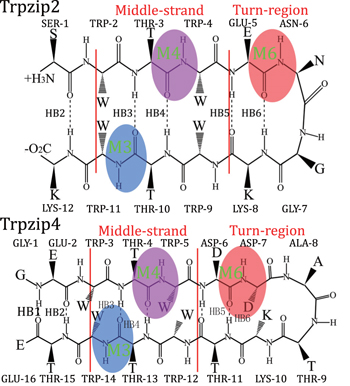
To further explore the capabilities of the isotopic Fourier transform IR (FTIR) and 2DIR melting spectra, we adapted this simulation protocol to identify the differences in peptide folding behaviors. Two hairpin polypeptides, Trpzip2 and Trpzip4, ^{[ 81 ]} with similar structures were compared (schematic structures for these two peptides are shown in Fig. 4 ). The previous simulation performed by Gao et al . ^{[ 45 ]} suggested that these two peptides have different folding mechanisms (“hydrogen-bond centric” for Trpzip2 and “hydrophobic core centric” for Trpzip4). Different folding landscapes of these two peptides were also suggested by some other simulation studies. ^{[ 30 , 48 , 82 – 84 ]} These comparisons demonstrate that certain spectroscopic features can be used to detect the difference in folding landscapes for these two peptides, but not to determine which folding landscapes are more realistic. In our simulated spectra, ^{[ 39 ]} different temperature dependences of intensities and ellipticities were observed for each isotopelabeled peak between the two peptides. Further analysis was performed to relate these spectroscopic observations to the different local structure stability patterns and thus to the different folding landscapes. ^{[ 39 ]} Our comparison suggested that the differences in folding behaviors of these two peptides are sensitively reflected by the ellipticity of the isotope peaks. ^{[ 39 ]} This is consistent with the conclusion that anti-diagonal width is a useful lineshape character to distinguish between the solvent exposed and the internal site, as suggested by Jansen et al . ^{[ 13 ]} To the best of our knowledge, this is the first example of this kind of theoretical spectroscopic analysis and the prediction is done based on the comprehensive peptide conformation samplings at a series of temperatures. ^{[ 38 , 39 ]}

Simulated thermal unfolding FTIR and 2DIR spectra of Trpzip2 peptide, with the temperature range of 285–350 K, are presented in Fig. 2(a) . Different C ¹³ isotope labeling schemes in our simulation, as demonstrated in Fig. 1 , were constructed to model the thermal unfolding spectra and to directly compare with experimental results. As demonstrated in Fig. 2(a) , at 285 K, the simulated linear absorption spectra of each isotopolog, an apparent peak υ _⊥ appears at 1635 cm ⁻¹ , a shoulder υ _|| at 1662 cm ⁻¹ , and a small peak or shoulder υ _iso were induced by the isotope labeling over the frequency range of 1580–1620 cm ⁻¹ . The line shapes of linear absorption spectra reasonably resemble the experimental observations in Ref. [ 48 ].

Fig. 1.

Figure Option View Download New Window

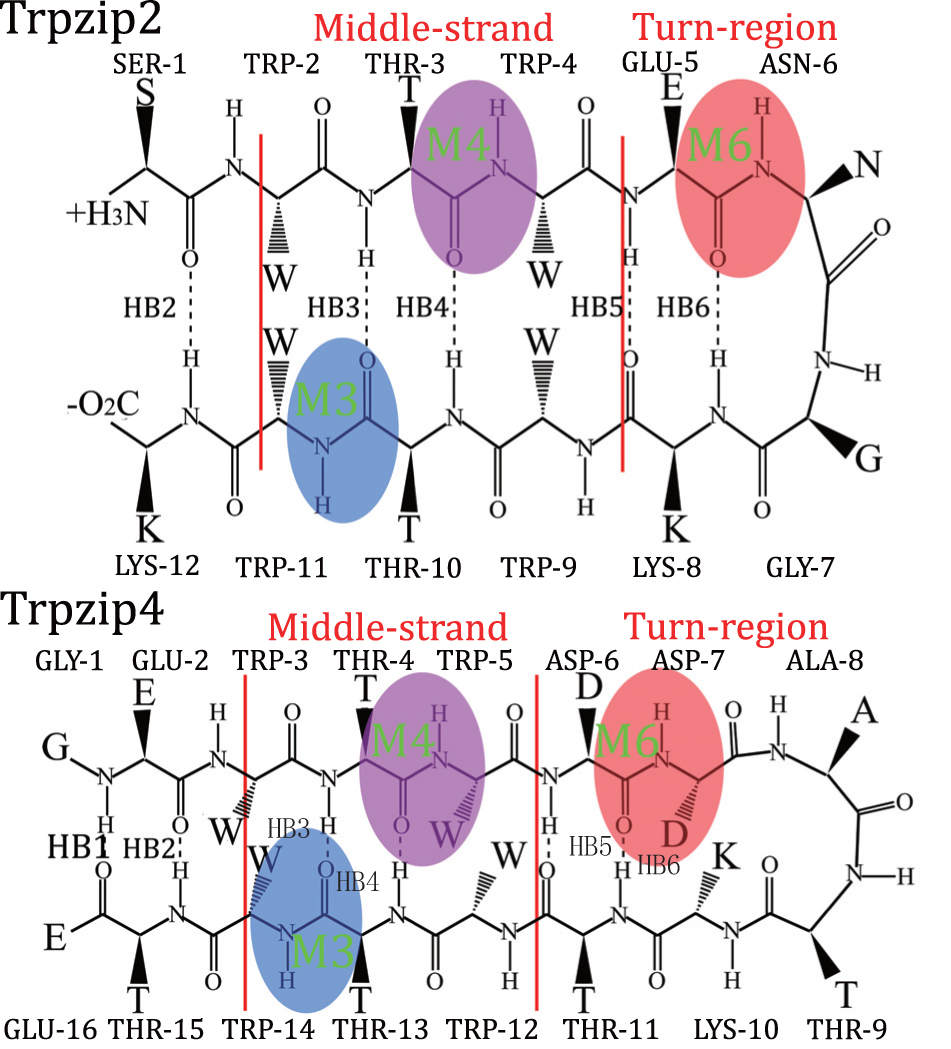Fig. 1. Structure of Trpzip2 (top row) with the isotope-edited sites TER- 1 (green), Mid-3 (blue), Mid-D (magenta), K-8 (yellow), and Turn-6 (red) highlighted, and Trpzip4 (bottom row), just the isotopologs Mid-3 (blue), Mid-D (magenta), and Turn-6 (red) in peptide were highlighted. The amide-I mode for these three isotope-edited sites in each polypeptides are also highlighted: M3, M4, and M6. The backbone hydrogen bonds HB2–HB6 are also labeled.

Fig. 2.

Figure Option View Download New Window

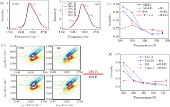
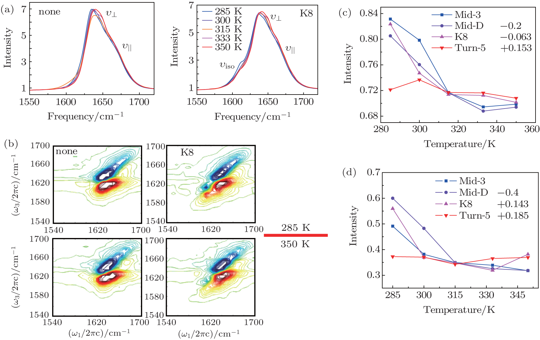Fig. 2. (a) Temperature-dependent simulated equilibrium FTIR spectra of isotope-unlabeled and isotopolog K8 in Trpzip2 taken from 285 to 350 K. Line color shows progression from blue to red. (b) The simulational 2DIR spectra of isotope-unlabeled and isotopolog K8 in Trpzip2 at 285 and 350 K. (c) Temperature-dependent intensities of the isotope-shifted peaks in the FTIR of different isotopologs. The curves of Mid-3, K8, and Turn-5 are shifted for better comparison. (d) Temperature-dependent intensities of the isotope-shifted peaks in the 2DIR spectra of different isotopologs. The curves of Mid-3, K8, and Turn-5 are shifted for better comparison.

As temperature rises, each isotopolog has a significant blue shift for the domain peak υ _⊥ , while the shoulder υ _|| shows no frequency shift. The simulated 2DIR spectra for each isotopologue are demonstrated in Fig. 2(b) . The signal of the unlabeled Trpzip2 shows a “Z”-shaped feature, consistent with the experiments, ^{[ 48 ]} which has been assigned as the feature of the β -hairpin. The 1635 cm ⁻¹ peak at 285 K blue-shifts to 1642 cm ⁻¹ at 350 K. The shoulder at 1660 cm ⁻¹ does not change as temperature increases, while the signal contour becomes more homogeneously broadened. Overall, the simulated temperature dependence of isotope-labeled FTIR and 2DIR spectroscopic features resembles the experimental observations. ^{[ 38 , 48 ]}

The temperature-dependent intensities of the isotope-labeled peaks are presented in Figs. 2(c) and 2(d) . The temperature-dependent intensity of each isotopolog in the linear absorption spectra presents significant and site-specific changes below 315 K, while above that a fairly concerted change is observed. This trend is more clearly observed for the intensity of isotope-shifted peaks in 2DIR spectra. ^{[ 38 ]} A similar phenomenon is also experimentally observed with the concerted change starting at 326 K; ^{[ 48 ]} the temperature difference between experiment and simulation should be consistent with the deviation between melting points observed in the other. The change of local environments can be considered as an incentive to the changes of peak intensity. A collective conformational change at higher temperatures, similar to the stability analysis of the backbone hydrogen bond, was concluded by the concerted intensity variations for all isotope-labeled peaks after 315 K. ^{[ 38 ]}

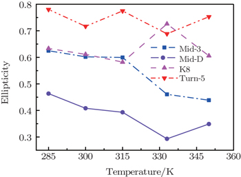
Value of ellipticity reflects the environment fluctuation around the amide-I mode. Ellipticity of a peak in the 2DIR spectra can be calculated as E = ( σ ² − Γ ² )/( σ ² + Γ ² ), ^{[ 85 , 86 ]} in which the diagonal line-width σ reflects inhomogeneous broadening, and the antidiagonal width Γ reflects the homogeneous broadening. Temperature-dependent ellipticities of the isotope-shifted peaks in the 2DIR spectra of different isotopologs were demonstrated in Fig. 3 . A clear drop in ellipticity is observed for the isotopologs of mid-strand mode related peaks Mid-D and Mid-3, which indicates that the mid-strand mode becomes more homogeneously broadened as temperature increases. The peaks related to the ellipticities of the turn modes such as K8 and Turn-5, however, do not show significant changes with increasing temperature. To further analyze the molecular origins of ellipticity differences, we analyze the static frequency distributions and time correlation functions of isotope-shifted frequencies for Mid-3 and Turn- 5. The time correlation function of Mid-3 decays faster with increasing temperature (118 fs vs 130 fs), while the time correlation function of Turn-5 decays at the same rate as the temperature rises; these should lead to the ellipticity drop. The static frequency distributions for both Mid-3 and Turn-5, however, show a small change as temperature increases. Similar to experimental observations, the intensities and ellipticities of the isotope-shifted peaks related to the mid-strand modes (Mid-3, Mid-D) show stronger temperature dependence compared with the turn modes, K8 and Turn-5; this suggests that Trpzip2 follows the “hydrogen-bonded centric” folding mechanism.

Fig. 3.

	Figure Option View Download New Window
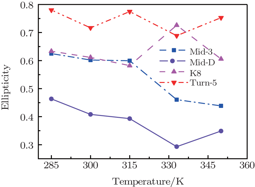	Fig. 3. Temperature-dependent ellipticities of the isotope-shifted peaks υ iso in the 2DIR spectra of different isotopologs.

Using the techniques developed, we further demonstrated that the different folding landscapes of two beta hairpin polypeptides with similar structures, Trpzip2 and Trpzip4, can be discriminated by the thermal unfolding vibrational spectra. Three C ¹³ isotope labeling schemes, as presented in Fig. 1 , were performed for both peptides to observe the temperature-related variations of difference spectral features. The first scheme Mid-3 (blue) labels the residue THR-10 in Trpzip2 and residue THR-13 in Trpzip4 (related to HB3), and the related local vibrational mode was named M3. The second scheme Mid-D (magenta) double labels the residues (THR-3 and THR-10) in the middle of Trpzip2 and THR-4 plus THR-13 in Trpzip4 (related to HB3 and HB4), and the related local vibrational mode (THR-3 in Trpzip2 and THR-4 in Trpzip4) was named M4. The last scheme Turn-6 (red) labels the residues in the turn-region: GLU-5 in Trpzip2 and ASP-6 in Trpzip4 (related to HB6); the mode located on GLU-5 in Trpzip2 and ASP-6 in Trpzip4 was named M6.

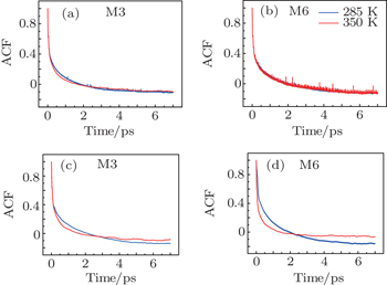
The time correlation function of the local amide-I modes M3 and M6 are demonstrated in Fig. 4 . As temperature increases from 285 to 350 K, for Trpzip2, the mid-strand mode M3 has a large decrease in relaxation time, from 130 to 118 fs, while the relaxation time of the turn mode M6 hardly changes. This indicates that the turn region has a lower thermal dependence compared with the mid-strand. For Trpzip4, however, the relaxation time of M3’s TCF decreases from 406 to 220 fs, while that of M6’s TCF decreases from 440 to 189 fs with temperature rising from 285 to 350 K. The relaxation time of M6’s TCF shows greater change compared with that of the M3’s, which suggests a lower thermal stability. The relaxation times of the TCFs for M3 and M6, apparently, are more sensitive to structural changes and thus to the local thermal stability. After a local region is unfolded, its structure experiences a larger extent of fluctuation and more exposure to the solvent, which induces a faster relaxation of frequency fluctuation.

Fig. 4.

	Figure Option View Download New Window
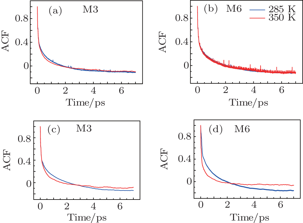	Fig. 4. Frequency-time correlation functions of the localized amide-I modes ((a), (c) M3 and (b), (d) M6) for Trpzip2 (top row) and Trpzip4 (bottom row) at 285 and 350 K, respectively.

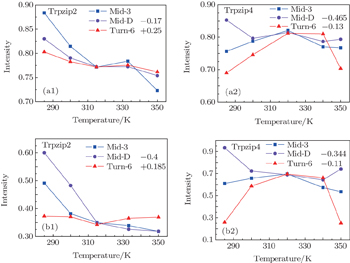
The temperature-dependent intensities of the isotope-labeled peak or shoulder in the linear absorptions of all the three isotopologs are presented in Fig. 5(a) for each peptide. For Trpzip2, both the isotope-shifted intensities of Mid-3 and Mid-D decrease while the intensity of Turn-6 has a much stronger temperature independence as temperature increases from 285 to 350 K. For Trpzip4, conversely, the isotope-shifted peak intensity of Turn-6 has the most significant and non-monotonic temperature dependence, while the intensities of both Mid-3 and Mid-D are highly stable.

Fig. 5.

Figure Option View Download New Window

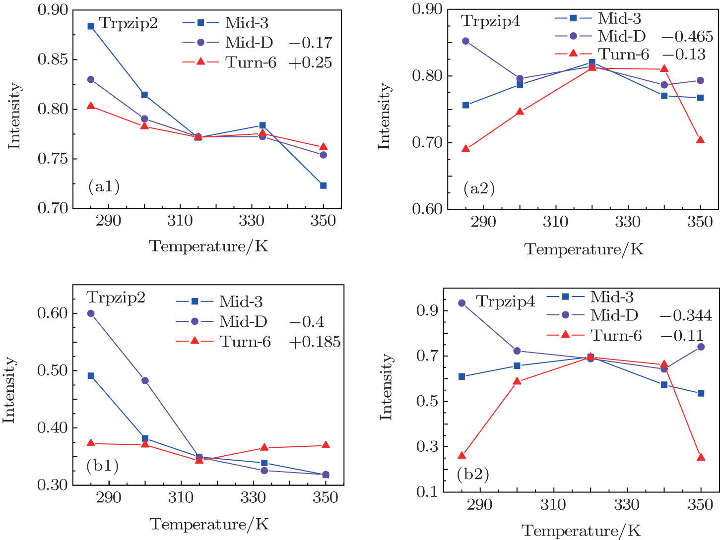Fig. 5. (a1), (a2) Temperature-dependent intensities of the isotope-shifted peaks υ iso in the linear absorption spectrum of different isotopologs. Both the curves of Mid-D and Turn-6 are shifted for better comparison. Temperature-dependent intensities of the isotope-shifted peaks υ iso in the 2DIR spectra for Trpzip2 (b1) and Trpzip4 (b2). The curves of Mid-D and Turn-6 are shifted for better comparison.

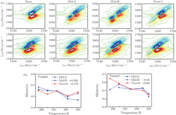
The 2DIR spectra of the unlabeled (none) and each isotopologue for both Trpzip2 and Trpzip4 polypeptides at 285 K are presented in Fig. 6(a) . The unlabeled 2D spectrum for Trpzip2 shows a growing cross peak in the off-diagonal region with increasing temperature. As in the linear absorption spectra, the isotope-shifted intensity of Turn-6 in Trpzip4 shows a large fluctuation with increasing temperature, while the intensities in Mid-3 and Mid-D are rather invariant with temperature. The temperature-dependent intensities of the isotope-labeled peaks in the 2DIR signals are demonstrated for all the isotopologs in Fig. 5(b) . For Trpzip2, on the other hand, the intensity of the isotope-labeled peak in Turn-6 presents higher temperature stability than Mid-3 and Mid-D.

Fig. 6.

	Figure Option View Download New Window
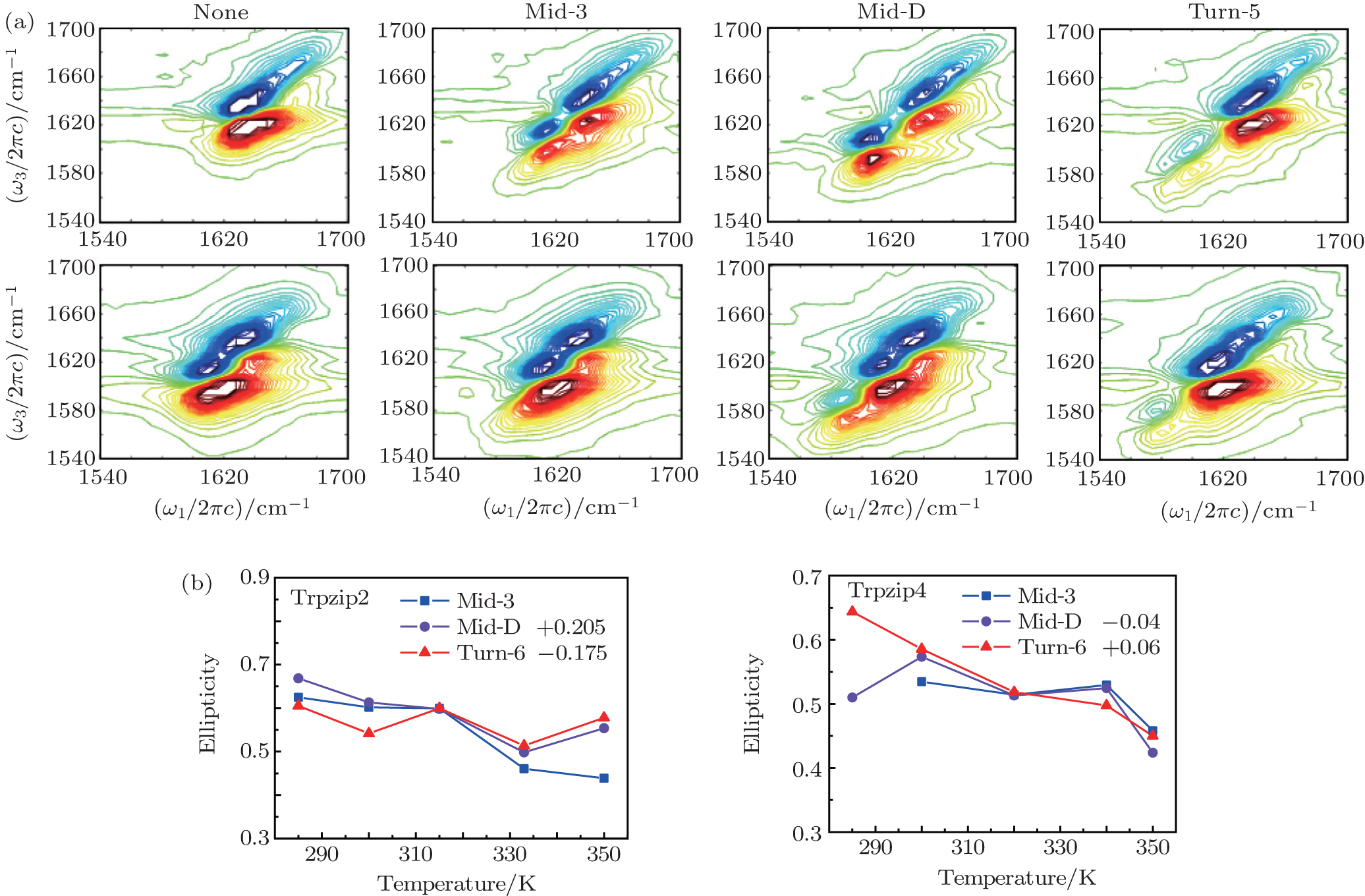	Fig. 6. (a) 2DIR spectra of each isotopologue for both Trpzip2 (above) and Trpzip4 (below) are recorded at 285 K in simulation. (b) Temperature-dependent ellipticities of the isotope-shifted peaks in the 2DIR spectra of different isotopologs for Trpzip2 (left) and Trpzip4 (right). The curves of Mid-D and Turn-6 are shifted for better comparison.

The isotope-labeled peak intensities of both FTIR and 2DIR demonstrate that different regions in Trpzip2 and Trpzip4 have different temperature dependencies. The isotope-shifted M6 peak in Turn-6 has the minimum intensity change in Trpzip2, and the maximum in Trpzip4. Other characteristics like the frequency distribution of vibrational modes, isotope-labeled peak shift, and full-width and half-maximum (FWHM), are not very sensitive to the local thermal stability. Furthermore, the intensity change of Turn-6 in Trpzip4 is non-monotonic. The intensity, therefore, is not aninformative marker for changesin local structure.

Temperature-dependent ellipticities of the isotope-labeled peaks of the 2DIR signals are presented in Fig. 6(b) for both peptides. The ellipticity of the isotope-labeled peak in Turn-6 in Trpzip2 shows much higher temperature stability than other isotopologs (Mid-3 and Mid-D). For Trpzip4, however, the ellipticity of isotope-shifted peak in Turn-6 decreases more significantly than that in Mid-3 and Mid-D as temperature increases.

The frequency distribution FWHM of the M3 and M6 modes are mostly constant as temperature increases. Therefore, the inhomogeneous broadenings of the isotope-labeled peaks are rather temperature-independent. The ellipticity is strongly correlated tovariations of the homogeneous broadenings, which are largely decided by the relaxation times of the frequency TCFs. The mid-strand segments in Trpzip2 peptide unfold first and thus the local environments around the M3 and M4 modes present much larger fluctuations compared to those around M6 in the turn-region. This difference in local structure stability induces a larger change in the frequency TCF relaxation time for the vibrational mode M3 than that for M6, and consequently a larger decrease in ellipticity. For Trpzip4, conversely, the local stability around M6 at the turn segment decreases more sharply than those around M3 and M4 at the mid-strand with increasing temperature, and eventually ellipticity presents a larger decrease for the Turn-6 isotopologue. Due to the sensitivity to homogeneous broadenings, the ellipticities of the isotope peaks in the 2DIR signals are more sensitive to these local stability differences than other spectral features like peak intensities; this suggests that the different folding landscapes for Trpzip2 and Trpzip4 polypeptides, the “hydrogen-bonded centric” and “hydrophobic-core centric” folding mechanisms, respectively.

We propose a cost-effective protocol to simulate FTIR and 2DIR spectra for polypeptides at a series of temperatures, based on comprehensive configuration samplings generated using implicit-solvent MD simulation combined with the ITS method, which provide an accurate thermal spectroscopic description consistent with experimental observables. Furthermore, to distinguish the differences inmelting spectra descriptions of peptide-folding behaviors, this protocol was adapted to simulate the thermal unfolding spectra for two β -hairpin peptides, Trpzip2 and Trpzip4, which were suggested to have different folding mechanisms. Comparison of the temperature-dependent signals for these two peptides, and the ellipticities of the isotope-labeled peaks were suggested to be more informative about the folding landscape differences, due to their sensitivity to homogeneous broadenings. Combined with the relevant experimental measurements, these modeling techniques can provide a better understanding of the peptide folding landscapes.

The amide-I vibrational band, although achieving great success in revealing secondary structure motifs of proteins, appears less sensitive to finer structural differences. For these “beats” differences, the amide III band, which mainly comprises backbone C–N stretching and N–H bending and is more delocalized than the amide I band, could be a potential solution. Moreover, the NEP method proposed here can work for any nonlinear optic process, including the surface-specified spectroscopy of sum frequency generation. Our next step will be to focus on using the NEP method together with the amide III band to investigate protein configuration dynamics in various chemical environments, which may help obtain a deeper understanding of fundamental life processes, like ion channels and photosynthesis. To further improve the current protocol, more close collaborations between the experimentalists and theorists are required.