1. Introduction Biological systems are typically complex nonequilibrium systems across many scales, ranging from the function and recognition of proteins, [ 1 – 7 ] to the cellular networks of macromolecular complexes and regulatory pathways, [ 8 – 21 ] and even the populations of organisms. [ 22 – 24 ] A biological system usually consists of a complex network of components working together to perform specific functions shaped by evolution. The function of a biological system resides not only in the individual components, but also, more importantly, in their interactions and collective behaviors. The challenge is how to explore the complex dynamics of nonequilibrium biological systems and uncover the underlying physical mechanisms. Various experimental, theoretical, and computational approaches have been developed to meet the challenge. [ 9 – 21 , 23 – 39 ]
Physical and mathematical modeling of biological systems can give a quantitative description of the dynamical behavior of biological processes. [ 3 – 5 , 8 – 11 ] It complements intuitive observations and limited resolutions of experimental investigations. Ordinary differential equations can be used to model the deterministic dynamics of biological systems. For a system under the influence of stochastic fluctuations, which is typically the case for biological systems, Langevin and Fokker–Planck equations are usually able to reasonably describe the system’s stochastic dynamics. [ 8 – 11 , 40 – 43 ] With appropriate tools of statistical mechanics, the energy landscape theory offers a quantitative global approach to investigate the structure, function, and behavior of biological systems. Quantitative results and predictions from the energy landscape theory have been confirmed by both laboratory experiments and detailed simulations. [ 1 – 8 ] The landscape and flux theory, as a further development and an important extension of the energy landscape theory, brings out the indispensable role of the curl flux in nonequilibrium systems complementary to the potential landscape, which facilitates the unveiling of fundamental principles and physical mechanisms governing nonequilibrium biological systems with complex behaviors and varied functions across multiple scales.
On the molecular scale, the puzzle of how a denatured protein refolds to its native state (the Levinthal’s paradox [ 44 ] ) has been resolved by the funnel-like energy landscape. [ 1 – 7 ] The concept of funneled energy landscapes goes beyond the folding of protein monomers. Binding processes of biomolecules also have funneled landscapes whose topographies determine the binding mechanisms. [ 2 , 45 – 47 ] Protein folding can be regarded as a diffusion process on the energy landscape which eventually reaches the native state. As a result, the folding thermodynamics and kinetics can be inferred from the knowledge of the energy landscape. The energy landscape theory has been been further extended and applied to protein binding and conformational dynamics. [ 26 , 48 – 50 ] Significant progresses have been made on interpreting the results from the energy landscape perspectives. [ 51 – 53 ] Hence, the energy landscape theory gives a quantitative description with physical insights into the dynamics at the molecular level and has enhanced our knowledge of the corresponding biological processes.
In order to have a concrete understanding of the en-ergy landscape concept, we have used molecular dynamics simulations and equilibrium statistical mechanics to quantify the energy landscape of protein folding and binding dynamics. [ 29 , 54 , 55 ] The connections between theories and experiments have been established with quantified energy landscapes. We have explored a wide variety of models based on the energy landscape theory to investigate various biomolecular dynamics, including multi-domain protein folding, [ 56 ] intrinsically disordered proteins’ (IDPs’) binding–folding, [ 57 – 62 ] and protein conformational changes. [ 63 – 68 ] The simulation results are consistent with the experiments in many ways, identifying the critical role of the energy landscape in biological processes.
Further, the energy landscape theory allows us to use bioinformatics input to learn the rules of energetic interactions that govern protein folding and ligand binding. The energy landscape theory has been used to quantify not only the affinity but also the specificity for molecular recognition critical for drug discovery. [ 26 , 28 , 69 – 71 ] Protein structures and binding complexes have been predicted successfully using optimized energy functions based on the energy landscape theory. [ 26 , 28 , 30 – 38 , 69 – 71 ]
At the scales encompassed by systems biology, research on the dynamics, function, and stability of nonequilibrium biological networks has progressed. [ 9 – 19 , 23 , 24 , 39 – 41 , 72 – 78 ] In particular, the landscape and flux theory, which we have developed and applied to explore a variety of biological systems, is our contribution to the advancement of this field. [ 9 – 19 , 23 , 24 , 39 ] The general theoretical framework of landscape and flux consists of several components inherently interlinked by the central idea of the driving force decomposition for nonequilibrium dynamical systems. We have discovered that, in contrast to the equilibrium dynamics of biological systems determined only by the potential landscape, there are two essential parts that constitute the driving force of nonequilibrium biological systems: the gradient potential force and the curl flux force. More specifically, the potential here means the nonequilibrium potential landscape quantifiable via the steady-state probability distribution, and the flux refers to the steady-state probability flux, a signature of detailed balance breaking that indicates the system’s nonequilibrium feature in the steady state. Both parts are required to give a complete characterization of the nonequilibrium dynamics of biological systems. Based on the driving force decomposition, other components in the landscape and flux framework, including the nonequilibrium thermodynamics, the fluctuation–dissipation theorem, the fluctuation theorem, the gauge field, and the path integral with kinetic paths and rates, become integral parts of a coherent theoretical framework.
We have applied the general landscape and flux framework to investigate a wide range of more specific nonequilibrium systems with biological significance. [ 9 – 12 , 14 , 16 , 18 , 19 , 22 – 24 , 39 ] In the investigation of the cell cycle process, cell cycle phases and cell cycle checkpoints have been identified, respectively, as the local attractor basins on the landscape and the transition states between them, along the path of cell cycle oscillation. [ 9 – 11 ] The Waddington landscape and path for stem cell development, differentiation, and reprogramming have been quantified in the landscape and flux framework. [ 12 , 14 , 16 , 18 , 19 ] Cancer has been proposed to be a disease of cellular states associated with the underlying gene regulatory network, where the multiple cellular states are identified as the attractor basins on the landscape; we have studied the transitions between the normal state and the cancer state quantitatively. [ 39 ] From the perspective of the landscape and flux theory, evolution dynamics that goes beyond Wright and Fisher has been formulated and the red queen phenomennon has been explained. [ 23 ] Ecosystems have also been investigated in the landscape and flux framework, with the global stability of ecological systems quantified. [ 22 ] Neural networks with asymmetrical connections have been studied for learning and memory. [ 24 ] In addition, the non-adiabatic dynamics of gene expression, [ 17 ] self regulating genes, [ 17 , 79 ] chaotic strange attractor, [ 80 ] and spacial development with pattern formation [ 81 – 84 ] have also been explored.
The rest of this article is structured as follows. In Section 2, we discuss the folding, binding, and conformational dynamics of biomolecules in the framework of the energy landscape. In Section 3, we address the intrinsic specificity and kinetic specificity for ligand binding as well as their applications in drug discovery and design in the context of the energy landscape theory. In Section 4, we review the general theoretical framework of landscape and flux and explore its more specific applications in cell cycle, stem cell, cancer, evolution, ecology, and neural networks. The conclusion is given in Section 5.
2. Folding, binding, and conformational dynamics of biomolecules 2.1. Intrinsic energy landscape quantification of protein folding and binding Although the concept of an energy landscape is widespread, researchers in the field of molecular biology often use the energy landscape theory in a qualitative way. This is mainly due to the fact that the energy landscape, reflecting the delicate relationship of energy, entropy, and structural information, cannot be explicitly measured by experiments. On the other hand, experimental measurements, such as the thermodynamic temperature and kinetic rate, cannot be well predicted by theories. Consequently, the relationship between the topography of the energy landscape and the thermodynamics and kinetics of biomolecular dynamics is ambiguous. To meet the challenge, molecular simulation is proposed to serve as the meeting point, aiming to bridge the gap between theories and experiments.
Conventionally, molecular simulations are often performed under constant temperature, corresponding to the canonical ensemble. However, the energy landscape, which reflects the underlying intrinsic interactions of the system, is not supposed to be dependent on temperature explicitly. Therefore, one has to transform the temperaturedependent distribution of energies from the canonical ensemble ( n ( E , T )) into the micro-canonical ensemble ( n ( E )). This can be done using the Boltzmann relation n ( E ) ∼ n ( E , T ) e E / k B T , as encoded in the weighted histogram analysis method (WHAM). [ 85 ] The distribution of the micro-canonical ensemble, referring to the density of states, corresponds to the intrinsic energy landscape.
In theories, there are three quantities describing the topography of the energy landscape: [ 2 , 4 , 5 , 45 ] energy gap δ E between the native state and the average of non-native states, measuring the slope of the funnel; [ 86 , 87 ] energy roughness Δ E , quantifying the bumpiness of the funnel; entropy S , describing the size of the funnel. These three quantities result in a dimensionless ratio Λ , expressed as the energy gap versus energy roughness and entropy  . As a characteristic of the energy landscape topography, Λ is a physical quantity measuring the funneled quantity of the energy landscape. All the topography quantities of the energy landscape can be calculated directly from the density of states.
We quantified the intrinsic energy landscapes of protein folding and presented the quantitative funnel diagrams. [ 54 ] The relationship of energy, entropy, and structure can be illustrated quantitatively from the energy landscapes (Fig. 1 ). On the thermodynamic aspect, there are two critical temperatures controlling protein folding: one is the folding temperature T f , at which the folding and unfolding states are equal in probability; the other is the glass transition temperature T g , at which the system becomes frozen with folding stagnation. [ 88 ] For a foldable chain, the folding temperature has to be higher than the glass transition temperature. On the kinetic aspect, the kinetic efficiency is often represented as the folding rate. In practice, both the thermodynamic temperature and the kinetic rate can be measured explicitly by experiments.
We found that the energy landscape topography Λ has a strong positive correlation with the thermodynamic stability (versus glass trapping) and kinetic rate. In other words, a more funneled energy landscape leads to more stable folding and a faster rate. Thus we have established the quantitative relationship between an energy landscape and folding thermodynamics and kinetics.
We then quantified the energy landscapes of protein binding. [ 29 ] For flexible biomolecular recognition, the central issue that needs to be addressed is the binding mechanism. We picked out 15 different homodimers and classified them into two groups based on different binding mechanisms found by experiments: 2-state “coupled binding–folding” homodimers and 3-state “folding prior to binding” homodimers. By quantifying the individual binding, folding, and global binding–folding energy landscapes (Fig. 2 ), we found that the 3-state homodimer has a more significant folding-versus-binding energy landscape funnel than the 2-state homodimer. We proposed a ratio expressed as the energy landscape topography of binding versus folding, Λ bind / Λ fold , to measure the binding mechanism quantitatively. Thus we classified the binding mechanisms successfully through the quantified energy landscape approach.
By calculating the global binding–folding energy landscape topography Λ global , we found that Λ global is strongly correlated with the thermodynamics and kinetics of protein binding, similar to the situation in protein folding. Our findings show that the energy landscape controls the pathway, thermodynamic feasibility, and kinetic efficiency of protein to realize its function.
Using molecular simulations, we demonstrated the crucial role of the energy landscape in biomolecular dynamics. The thermodynamics and kinetics of protein folding and binding can be predicted well with the quantified energy landscape due to the strong correlation between them. On the other hand, with experimental measurements on thermodynamics and kinetics, the energy landscape can be portrayed accurately. These results bridge the gap between theories and experiments, providing a novel way to understand the biomolecular dynamics by combining the results from both theories and experiments.
2.2. Binding–folding free energy landscape quantification of intrinsically disordered proteins The long-standing paradigm that a biomolecular function is determined by a unique folded structure is challenged by intrinsically disordered proteins (IDPs). [ 89 – 91 ] An IDP lacks a unique tertiary structure in an isolated state, either entirely or in parts, but often folds upon binding to its partners. [ 92 , 93 ] This “binding induced folding” scenario gives IDPs many advantages, [ 94 , 95 ] including fast association/disssociation rate, multiple binding targets, low affinity but high specificity, etc, resulting in IDPs’ presence in many critical cellular activities, such as transcription, signaling, and regulation. [ 96 – 98 ] Understanding IDPs’ binding–folding will refresh our view on protein folding and contributes to our knowledge of molecular biology.
The structure-based model (SBM) is a simplified molecular simulation model, derived from the energy landscape theory. [ 99 ] The SBM only takes into account native interactions, leading to a perfect funneled energy landscape. The validity of SBM is supported by the “principle of minimal frustration” indicating that the native structural topography controls the folding mechanism, and also the increasing reports in which the simulation results are consistent with experiments in many ways. [ 27 , 99 , 100 ] IDPs’ binding–folding processes were investigated extensively by a coarse-grained SBM, [ 58 , 101 – 103 ] built on the basis of the final binding complex structure located at the bottom of the energy landscape, which reproduced the binding–folding mechanism very well in agreement with experiments. Huang et al . applied a plain coarse-grained SBM, which modulates the strengths of the native contacts, to examine the kinetic advantage of IDPs’ binding. [ 104 ] The thermodynamic free energy landscapes and kinetic rates were analyzed comprehensively from the simulation results. The analysis led to the conclusion that, compared to ordered chains, the flexibility in IDPs endows them with a stronger tendency to form the bound complex from an encounter complex with the partners, thus providing a practical explanation for the “flycasting” mechanism. [ 95 ]
Recently, we developed a two-bead SBM with explicit incorporation of electrostatic interactions to investigate IDP histone chaperone Chz1 binding–folding to histone H2A.ZH2B [ 60 ] (Fig. 3 ). By analyzing the interactions in the transition state ensemble, we found that the interactions are chargeoriented, indicating that the electrostatic interactions serve as the driving force at the early stage of the recognition, consistent with experiments. [ 105 ] We also found that Chz1 collapses to a non-native conformation at low salt concentration due to the strong intra-chain electrostatic interactions. Although the collapsed structures in IDPs are widely found in experiments, [ 106 – 108 ] their effects on IDPs’ function remain unclear. We found that it consumes time to unravel the collapsed structure in Chz1 during binding. Therefore, we proposed opposite roles of electrostatic interactions in IDPs’ binding–folding: the inter-chain interactions facilitate binding through the fly-casting mechanism, while the intra-chain interactions impede the binding via local collapsing or trapping. We argued that IDP itself is able to optimize the two effects to ensure its functional performance.
Although the coarse-grained SBM has made significant progress on the description of IDPs’ binding–folding processes, molecular simulation at the atomic level is in urgent need. However, due to the limit of computational resources, atomistic simulations are often focused on a class of small single-domain proteins on specifically-designed computers. [ 109 , 110 ] To overcome the difficulty, a variety of multi-scale molecular simulations were developed by combining the coarse-grained and atomistic simulations to explore biological processes at a wide range of spatial and temporal scales. We used a multi-scale molecular simulation approach combining coarse-grained SBM and atomistic optimal path calculation method to explore the binding–folding process of IDP inhibitor IA3 to its target enzyme (Fig. 4 ). [ 59 ] With the analysis of the kinetic data from laser temperaturejump fluorescence spectroscopy and fluorescence resonance energy transfer (FRET), experimentalists concluded that binding is prior to folding for IA3. [ 111 ] Our coarse-grained model generated thermodynamic free energy landscapes, which confirmed the binding mechanism. Further analysis on the contact map in the transition state underlined the important role of non-native interactions in the binding–folding process. With the quantified optimal pathways at the atomic level, we analyzed in detail the binding prior to folding mechanism by the formation of a helix in IA3 after going through significant nonnative interactions. We argued that the transient non-native interactions can shrink the entropy of the energy landscape, leading to an efficient binding–folding process.
With our recently developed hybrid all-atom model and multi-scale simulation approach, we explored the binding–folding process of an IDP in measles virus nucleoprotein ( α -MoRE) to its target. [ 61 ] α -MoRE, regarded as an IDP, forms a perfect α helix during its molecular recognition. [ 112 – 114 ] Experiments revealed that α -MoRE in solution is not an ideal random coil but in rapid interconversion between the unfolded state and multiple partially helix formed states. [ 115 ] We first set up an REMD simulation with a Charmm22* force field [ 116 ] to explore the inter-chain dynamics of α -MoRE in solution. Through clustering analysis, [ 117 ] we found that α -MoRE dominates at a series of partially helix formed clusters (Fig. 5 ), consistent with the experimental findings. Additionally, the simulations and experiments are strongly correlated by fitting chemical shift data, confirming the existence of the dynamic conformational equilibrium of α -MoRE in solution. Then we combined the empirical force field and the SBM potential together, constructing a novel hybrid SBM. The empirical force field describes the precise local-in-sequence interactions, aiming to capture the secondary formed structure in α -MoRE, while the SBM potential describes the non-local or long-range interactions, aiming to accelerate the recognition process in simulations. With quantified free energy landscapes, we proposed a “conformational selection followed by induced-fit” binding scenario for α -MoRE. We argued that this binding scenario will facilitate IDPs’ binding via a “kinetic divideand- conquer” mechanism to ensure a fast rate of association and dissociation, in favor of IDPs’ biological function.
The quantified multi-dimensional free energy landscapes along various reaction coordinates provide clear pictures on how the binding–folding process in IDPs occurs. Analyses from free energy landscapes, such as interactions and clustering, give comprehensive explanations on the role of nonnative interactions, collapsed structure, downhill folding, intrinsic disorder, and molten globule in IDPs’ biological function. Based on the energy landscape theory, SBM is sufficient to capture the characteristic of IDPs’ binding–folding, indicating that the theory can be applied to proteins with even weakly-funneled or anti-funneled energy landscapes.
2.3. Functional free energy landscape quantification of large-scale conformational dynamics Protein realizes its function by binding to its partners. During recognition, protein often undergoes largescale conformational changes to achieve its specific biological function. [ 118 ] Even in isolated states, protein does not always possess a single well-defined structure. Instead, protein often fluctuates among multiple states to facilitate its biological function, implying there are multiple basins on the energy landscapes. [ 48 , 49 , 119 , 120 ] To understand how protein realizes its function, it is essential to understand how functional structural rearrangements occur at the molecular level. Recent developments in experimental techniques, such as single-molecule and nuclear magnetic resonance (NMR) measurements, have improved our knowledge of biomolecular dynamics significantly. However, due to limited spatial and temporal scales, it is still challenging to characterize functional conformational dynamics experimentally. Hence, various molecular simulations have been developed to quantify free energy landscapes.
The basic strategy in simulation is to build a multi-basin SBM potential function. There are three classes of models at different levels: macroscopic model, [ 121 , 122 ] where multiple potentials, each of which has a single energy minimum unambiguously defined by a prior structure, are connected smoothly at the joined point, resulting in a multi-basin energy function; microscopic model, [ 63 – 65 ] where the elementary potential between two atoms in proteins is modeled to have multiple minima, corresponding to multiple structures; mesoscopic model or microscopic mixing contact map, [ 66 , 67 , 123 ] where individual energy terms (usually native contacts) from multiple structures are mixed separately with different mixing protocols.
We first focused on an excellent allosteric model, adenylate kinase (ADK), which is composed of a core domain (CORE), an ATP-binding domain (LID), and a nucleoside monophosphate binding domain (NMP). During its catalytic function, ADK undergoes large-scale domain arrangement from open to closed state. [ 124 , 125 ] To explore the conformational dynamics of ADK, both microscopic and mesoscopic models were investigated in our group. The microscopic model was developed to explore the intrinsic dynamics of ADK. [ 63 ] Using free energy landscapes and contact maps, we addressed the critical dynamical interplay between LID and NMP domain and characterized the hot residues controlling the intrinsic dynamics. Furthermore, the mesoscopic model developed recently with explicit consideration of substrates (AMP and ATP) has made a great contribution to the global understanding of intrinsic and functional dynamics in ADK (Fig. 6 ). [ 67 ]
Combining both models, we proposed that only with binding can ADK be induced to a dominate closed state, confirming the pivotal role of substrates on the functional dynamics of ADK. In addition, we found that there are two parallel binding pathways with two intermediates from the quantified energy landscapes. Based on the thermodynamic and kinetic results, we concluded that the motion of the NMP domain is the rate-limiting step for ADK’s conformational change. The remarkable degree of fluctuating intrinsic dynamics in ADK is supposed to favor the functional conformational changes during substrates binding.
Then we explored the functional dynamics of DNA Yfamily polymerase IV (DPO4) binding to its target DNA. [ 68 ] Structural analysis reveals that DPO4 exhibits distinct conformations in the apo and DNA bound state, implying that DPO4 undergoes a large-scale conformational transition during its binding to DNA. [ 126 ] Accordingly, we built a two-basin mesoscopic SBM, aiming to capture the details of flexible protein- DNA recognition. From thermodynamic free energy landscapes, we found that the DPO4-DNA recognition process undergoes four different kinetically connected stages: unbinding state (US), encounter complex (EC), intermediate state (IS), and binding state (BS) (Fig. 7 ). Furthermore, we found that at different stages, DPO4 itself has different conformational distributions among the apo state (A-state), DNA-bound state (B-state), and intermediate state (I-state). Therefore, we drew a dynamic picture of DPO4-DNA binding accompanied with the distributions of the DPO4 conformations varying at different binding stages. With the calculated kinetic rates at each step, we found that the conformational dynamics or flexibility in DPO4 contributes to the efficiency of DNA recognition. Intriguingly, DPO4 is still in the conformational equilibrium between I- and B-state at the final protein-DNA complex, leading to fluctuating interactions between protein and DNA. DPO4 is a typical Y-family polymerase, responsible for low-fidelity of DNA synthesis. [ 127 ] The flexible transient interactions between DPO4 and DNA may have implications on DPO4 accommodating the bypass of various DNA lesions. The theoretical investigations on DPO4 binding to DNA offer a unique insight on the conformational dynamics affecting the protein’s catalytic function.
Built on the energy landscape theory, the multi-basin SBM can explore the functional conformational dynamics in protein during its binding. The multi-basin model aims to capture the intrinsic conformational fluctuation in protein and its role in protein’s function. With the quantified free energy landscapes and kinetic rate/flux analysis, we can gain a global picture of the functional conformational dynamics, giving a deeper understanding of the protein dynamics.
3. Ligand binding specificity and drug discovery 3.1. The intrinsic specificity and its applications in drug discovery Specificity refers to the discrimination of the same ligand binding to its partner against other possible receptors (Fig. 8(a) ). In thermodynamics, it is the relative difference in the affinity between the specific binding complex and other competitive complexes. [ 128 – 131 ] In terms of Boltzmann distribution ( P ∼ exp[− F / k B T ]), the populations of different conformations depend on the binding free energy exponentially. As a result, the binding free energy gap between the specific complex and the competitive ones can result in a large population distinction in equilibrium. In practice, it is challenging to quantify this conventional concept of specificity since the receptor universe is too large and the information about them is usually limited.
To circumvent the challenge, an alternative way to determine quantitatively the ligand–receptor binding specificity was proposed. [ 26 , 28 , 36 ] In a thought experiment, one can assume that the N and C terminus of each protein receptor of the protein universe are connected by linkers. In this sense, multiple individual receptors connected by the linkers are equal to a single large composite receptor. The conventional specificity discriminating a ligand binding to a specific receptor against other receptors (Fig. 8(a) ) becomes the discrimination of a ligand binding to a specific site (mode) against other binding sites (modes) of the large composite receptor (Fig. 8(b) ). In other words, the large target receptor can be viewed as many small receptors linked together. In this way, the quantitative description of specificity refers to the gap of binding energy between the specific binding mode and other competitive binding modes, rather than the gap between the specific binding partner and other competitive binding complexes. Similarly, a receptor with diverse binding modes by a ligand (Fig. 8(b) ) is equivalent to that of the ligand universe binding to the same receptor (Fig. 8(c) ), under the assumption that the receptor is large enough. Thus, exploring the binding interactions via diverse sites of the receptor (Fig. 8(b) ) and exploring the binding interactions via sequences (diverse receptors in Fig. 8(a) or diverse ligands in Fig. 8(c) ) are equivalent. With the assumption of a large target receptor, one can term this criterion for specificity as the intrinsic specificity, in contrast with the conventional concept of specificity.
The process of receptor–ligand binding can be described and physically quantified by the funnel-like energy landscape, with the native binding mode at the bottom and the binding roughness located in the binding paths. [ 25 – 29 ] From the funnel-like energy landscape, the native conformation has the lowest binding energy (Figs. 9(a) and 9(b) ) and the energies of the non-native conformations are determined by the statistical Gaussian distribution (Fig. 9(c) ). A dimensionless quantity ISR (intrinsic specificity ratio) is proposed to quantify the magnitude of intrinsic specificity (Figs. 9(c) and 9(d) ), which is proportional to the ratio of the binding temperature and the trapping temperature ( T b / T g ). [ 26 ] The formula to calculate ISR is given by
where
α scales the entropy contribution

to the specificity; δ
E represents the gap between the native conformation
E N and the decoy ensemble 〈
E D 〉; and Δ
E represents the energy roughness of the decoys. Mathematically,


where 〈·〉 is the average over decoy ensemble. A larger ISR suggests a higher discrimination for the native binding state against the decoys, therefore a higher intrinsic specificity. ISR gives a quantitative description of the intrinsic specificity without assessing the conventional specificity that requires the exploration of the ligand or receptor universe.
It is known that specificity and affinity are both required for efficient and specific biomolecular recognition. However, most quantitative descriptions of biomolecular recognition were focused on improving the computation of affinity while lacking the quantification of specificity. Based on the intrinsic specificity and the corresponding intrinsic specificity ratio (ISR), [ 28 ] Liu et al . explored and characterized the binding modes of levamlodipine and human serum albumin (HAS), validating a high ISR value for the binding site of levamlodipine. [ 132 ] Furthermore, Wang et al . developed twodimensional computational drug screening considering both affinity and intrinsic specificity as the selection criteria. [ 28 ] By using the two-dimensional virtual screening with ISR and affinity, Wang et al . successfully identified three active hits against Ras protein. [ 133 – 137 ] Yang et al . further studied the target Ache using two-dimensional virtual screening for potential inhibitors. [ 70 ] Combined ligand screening of the shape and electrostatic similarity as well as local binding site similarity was also applied to search for known drugs against cognitive deficits. For the first time, we found that pazopanib, known as a tyrosine kinase inhibitor for cancer treatment, can inhibit acetylcholinesterase (AchE) activities at the sub-micromolar concentration.
To improve the accuracy of binding affinity prediction, Yan et al . developed the novel scoring functions of protein–ligand, protein–protein and protein–nucleic acid interactions, named SPA, [ 36 ] SPA-PP, [ 37 ] and SPA-PN, [ 38 ] respectively. The optimization strategy is to maximize the performances on intrinsic specificity and affinity predictions simultaneously by tuning the energy parameters according to the funnel-like energy landscape. In addition, Zheng et al . performed twodimensional virtual screening with ISR and affinity evaluated by the scoring function SPA [ 36 ] against flexible Ras protein and protein–protein interactions involving the Ras protein. [ 138 ]
3.2. The kinetic specificity and its applications in drug discovery In the equilibrium condition, the binding free energy in vitro can be computed by the kinetic rate constants according to the equation quantifying the relation between the kinetic constants and the thermodynamic features in vitro . However, the condition in vivo is usually a nonequilibrium condition. Consequently, the effectiveness of ligand binding may be affected not only by the thermodynamic properties, but also by the dissociation rate (off-rate constant) determining the residence time (half life). [ 139 , 140 ] The longer the residence time is, the more potent the drug is on the the receptor in vivo . Therefore, not only the thermodynamic affinity and specificity, but also the residence time of the drug on the receptor quantified as the kinetic specificity, determine the duration and effectiveness of the drug.
To calculate the residence time practically, a diffusion process on the energy landscape was used to model the ligand–receptor binding/unbinding kinetics. [ 141 ] In this way, the residence time can be obtained approximately from the kinetic time via the diffusion dynamics. The driving force of this process is determined by the gradient of the free energy landscape. By projecting the free energy onto a reaction coordinate or order parameter, the binding/unbinding kinetics on the energy landscape can be modeled by the following one-dimensional diffusion equation: [ 142 , 143 ]
where
P (
r ,
t ) is the probability distribution of the binding conformation with specific
r (RMSD, root mean square displacement) at time
t ,
D (
r ) denotes the diffusion coefficient which is in general a function of
r (for simplicity, we consider constant diffusion coefficient
D in the following calculation), and
F (
r ) represents the free energy of the binding system at a given
r . The residence time (RT) for the native binding conformation can then be calculated by integrating the above diffusion equation
At
r n = 0 where the system is in the native state, the reflecting boundary condition is imposed. At
r u where the binding is in the “non-native” states, the absorbing condition is used. Note that the choice of
r u is system-specific.
The kinetic specificity quantified by the calculated residence time showed moderate correlations with both thermodynamic stability and specificity, [ 141 ] indicating the thermodynamics and kinetics of ligand binding can be optimized simultaneously. Practically, the intrinsic specificity ratio ISR is less difficult to obtain computationally than experimentally. In contrast, the kinetic specificity is less difficult to obtain experimentally than computationally. The microscopic molecular modeling (molecular dynamics or Monte Carlo simulations) demands tremendous computational time. The coarsegrained diffusion approach here is relatively fast and provides qualitative/semi-quantitative results, although not as accurate as MD or Monte Carlo simulations. The connection of thermodynamics and kinetics bridges a gap in the understanding of drug efficacy. It is also helpful for drug discovery and design. In drug screening, both experimentally and computationally, efforts to identify new lead compounds often concentrated merely on the optimization of the affinity. [ 144 ] Such a strategy neglected the importance of kinetic and thermodynamic specificities. Based on the previous studies on two-dimensional virtual screenings relying on thermodynamic specificity and binding affinity against the Ras protein and Ache protein, Wang et al. have further developed three-dimensional virtual screening taking into account the residence time describing the kinetic specificity. In the drug–target binding system, what determines the residence time of a drug residing in its target is the gap of binding affinity between the native state and the transition state. [ 139 , 140 , 145 – 148 ] Therefore, improving the stability of the native state could decrease the drug potency in vivo , if the affinity change of the transition state is larger than that of the native state. Also, improvement of the affinity may decrease the thermodynamic specificity, if the affinity gap between the native and non-native modes is reduced. This demonstrates the importance of taking the thermodynamic specificity and kinetic specificity as additional criteria for drug discovery.
Based on the energy landscape theory, ISR as quantified thermodynamic specificity and the residence time as quantified kinetic specificity were both quantified computationally. [ 141 ] This gives a quantitative means to choose and optimize the lead compounds computationally with multi-dimensional drug screening strategy by considering both affinity and specificities. Yan et al . [ 69 ] has tested this strategy on the drug targets COXs. As seen in Fig. 10(a) , two- or three-dimensional drug screenings (E+ISR, E+RT, or E+ISR+RT) are superior to any single parameter in discriminating the target COX-2 against COX-1 when binding with the selective drugs for COX-2. In addition, three-dimensional screening shows more capability than twodimensional screening in discriminating COX-2 against COX- 1. Also, two- or three-dimensional drug screening enhances discrimination between the selective and non-selective drugs when binding onto COX-2 (Fig. 10(b) ). Therefore, it is promising to conduct multi-dimensional (such as two- or three-dimensional) drug screening and target identification by incorporating the thermodynamic and kinetic specificities as selection criteria, instead of using affinity alone. Specificity can be used as an indicator in addition to affinity in drug screening to avoid side effects and seek more specific lead compounds.
4. Landscape and flux theory and its applications to biological networks 4.1. Landscape and flux theory for nonequilibrium systems In general, biological systems are nonequilibrium dynamical systems with complex behaviors and varied functions. [ 9 , 10 , 13 , 15 , 40 – 43 , 72 – 78 ] The deterministic dynamics of a generic class of nonequilibrium biological networks can be mathematically modeled by a set of ordinary differential equations, which can be written in the compact form

where
ẋ is a short notation for d
x /d
t , the vector
x denotes the collection of variables characterizing the system state, and
F (
x ) is the driving force governing the system’s deterministic dynamics.
In reality, biological environments are noisy and full of intrinsic and external fluctuations. Taking into account the effects of fluctuations, the Langevin equation usually gives a reasonable description of the system’s stochastic dynamics [ 40 – 43 ]

In addition to the deterministic driving force
F (
x ), there is also the stochastic force
ξ (
x ,
t ). It has the statistical properties 〈
ξ (
x ,
t )〉 = 0 and 〈
ξ (
x ,
t )
ξ T (
x ,
t ′)〉 = 2
ɛ D (
x )δ (
t −
t ′), where
ɛ is a scale factor characterizing the fluctuation strength (not necessarily small) and
D (
x ) is the diffusion matrix characterizing the fluctuation correlations.
[ 40 – 43 ] Corresponding to the stochastic dynamics described by the Langevin equation which traces a stochastic trajectory, the probability distribution evolves according to the Fokker–Planck equation (or diffusion equation), which in Ito’s prescription reads [ 40 – 43 ]
Interpreting this equation as a continuity equation
∂ t P (
x ,
t ) +
∇ ·
J (
x ,
t ) = 0, which represents the probability conservation, the probability flux is identified as

In the long time limit, in general, the system settles in the steady state,
P ss (
x ), which does not vary with time:
∂ t P ss = 0.
[ 40 – 43 ] Accordingly, the steady-state probability flux satisfies
∇ ·
J ss = 0, namely, the divergence-free condition. There are two physically distinct ways for
J ss to have vanishing divergence. One way is that the steady-state flux itself is zero,
J ss = 0, which indicates no flux in or out of the ensemble and characterizes the equilibrium condition satisfying detailed balance.
[ 40 – 43 ] The other way is that the steady-state flux
J ss itself does not vanish although its divergence is identically zero. Nonvanishing steady-state probability flux
J ss quantifies the nonequilibrium characteristics of the steady state with detailed balance broken.
[ 9 , 10 , 40 – 43 , 83 ] Due to the divergence-free condition,
J ss has a curl nature; its field lines typically circulate in loops (though they can also extend into infinity).
Applying Eq. ( 9 ) to the steady state, the driving force decomposition follows [ 9 , 10 , 83 , 149 ]

where
U = –ln
P ss is the potential landscape and
V ss =
J ss /
P ss is the flux velocity. Thus the driving force of nonequilibrium dynamical systems is decomposed into three parts: the gradient-like force of the potential landscape
U related to the steady-state probability distribution
P ss ; the curl-like force of the flux velocity
V ss connected to the steady-state probability flux
J ss ; and the fluctuation-induced force arising from the dependence of fluctuations on state variables, which disappears when
D does not depend on
x . For equilibrium systems, in which
J ss and thus
V ss vanish, the equilibrium potential landscape characterizes the system’s global stability of the system, while the gradient of the landscape determines the system’s dynamics. For nonequilibrium systems, in which
J ss and thus
V ss do not vanish, the nonequilibrium potential landscape characterizes the system’s global stability, while both the gradient force of the potential landscape and the curl force of the flux velocity determine the system’s dynamics.
In the small fluctuation regime, the stochastic dynamics of the system can be investigated using the WKB method. The Fokker–Planck equation is expanded in terms of the fluctuation strength parameter ɛ . The zero-fluctuation limit results in the following Hamilton–Jacobian equation: [ 22 , 23 , 41 , 83 , 150 ]

where
ϕ 0 = (
ɛ U )|
ɛ →0 is called the intrinsic potential. Following the deterministic dynamics
ẋ =
F , it can be shown that
ϕ 0 decreases monotonically with time

The equality holds when
∇ ϕ 0 = 0, i.e.,
ϕ 0 has reached its extremum. This means
ϕ 0 is a Lyapunov function, well suited to studying the global stability of deterministic nonequilibrium systems.
[ 22 , 23 , 41 , 83 , 150 ] Moreover,
V ss can also be expanded in terms of the fluctuation strength
ɛ . The leading order is shown to be
V 0 =
F +
D ·
∇ ϕ 0 ,
[ 22 , 23 , 83 , 150 ] where
V 0 =
V ss |
ɛ →0 = (
J ss /
P ss )|
ɛ →0 is the intrinsic flux velocity. Equation (
11 ) shows that

which means the gradient of the intrinsic potential and the intrinsic flux velocity are perpendicular to each other. In the zero-fluctuation limit, the driving force decomposition, in terms of the intrinsic potential
ϕ 0 and the intrinsic flux velocity
V 0 , reads
[ 22 , 23 , 41 , 83 , 150 ] 
Hence, both the intrinsic potential landscape and the intrinsic flux velocity contribute to the deterministic dynamics of nonequilibrium systems. Furthermore, the dynamical decomposition of the driving force into the potential landscape and the flux velocity has been further generalized to accommodate transient processes, time-dependent external conditions, multiple state-transition mechanisms, and spatially extended systems, of which we refer to Refs. [
82 ] and [
83 ] for a more complete presentation.
Based on the potential–flux dynamical decomposition, we investigated and extended the fluctuation–dissipation theorem, nonequilibrium thermodynamics, and gauge field formulation. [ 15 , 83 ] When generalized to the nonequilibrium regime, [ 15 , 151 – 154 ] the fluctuation–dissipation theorem for an observable Ω and perturbation on component i of the driving force reads [ 15 ]


where
∂ i ≡
∂ /
∂ x i ,

is the effective driving force, and
V k =
J k /
P is the transient flux velocity.
[ 83 ] The Einstein notation of summing over repeated indices is used. 〈·〉 represents the average over the ensemble distribution
P . We have also set
ɛ = 1 (the same as below unless specified otherwise). Note that the probability flux (velocity) defined here in the Fokker–Planck equation differs from that used in Ref. [
15 ] by a minus sign (the sign used here agrees with the convention in physics). The left-hand side of the equation is the response function of the observable to perturbation. On the right-hand side of the equation, the first term is the correlation function of the observable with the effective driving force, representing the fluctuation properties of the system (similar to the equilibrium case); the second term arises from the flux force breaking detailed balance which characterizes the nonequilibrium condition (including the nonequilibrium transient process).
[ 83 ] To make contact with the nonequilibrium thermodynamics, we choose the observable Ω = V i and take the equal time limit t = t ′ in Eq. ( 15 ), which gives [ 15 ]

where the index
i is also summed over. The left side is the rate of change of system entropy

. The first term on the right (without the minus sign) is identified as the rate of entropy flowing from the system to the environment

. Its relation to the average heat dissipation rate in the environment (medium) is given by

when the environmental temperature
T is constant. The second term on the right, which is non-negative, is identified as the entropy production rate
, driven by the flux velocity. Therefore, equation (
16 ) can be interpreted as the entropy balance equation

.
[ 15 , 83 ] Further, taking the observable as the relative flux velocity  [ 83 ] and following similar procedures as above, we obtain [ 15 , 83 , 151 – 154 ]
where

is the nonequilibrium free energy defined as

, with the nonequilibrium internal energy

. These definitions apply when the environmental temperature is constant and there are no time-dependent external conditions.
[ 83 ] The first term on the right side is the total entropy production rate

. The second term, which is non-negative, is identified as the adiabatic entropy production rate

. It is related to the house keeping heat via

when the environmental temperature is constant. The term on the left side,

, is also non-negative and identified as the non-adiabatic entropy production rate
. Hence, equation (
17 ) can be interpreted as the entropy production decomposition equation

.
[ 83 ] The entropy production rate can be decomposed into the contribution of spontaneous relaxation to the steady state from the transient state and that of detailed balance breaking in the steady state driven by the steady-state flux sustaining the nonequilibrium environment.
[ 15 , 83 , 155 – 158 ] Moreover, a more general set of nonequilibrium thermodynamic equations, taking into account time-dependent external conditions, can be constructed directly from the potential–flux dynamical decomposition, which includes the above two equations as special cases [ 83 ]

where

,

,

,

and we have adapted the notations to those used here. The effect of time-dependent external conditions is represented by the thermodynamic power (work per unit time)

. A further extension of this set of equations and its application in a spatial stochastic neuronal model can be found in Ref. [
83 ].
The connection to the gauge field theory [ 15 ] is realized by the covariant derivative ∇ i = ∂ i + A i , with the gauge field identified as  . The probability flux can be rewritten as J i = − D ij ∇ j P . Associated with the Abelian gauge field A i , there is an internal space with curvature R i j = [ ∇ i , ∇ j ] = ∂ i A j − ∂ j A i . R i j is gauge invariant, meaning for a gauge transformation A i → A i + ∂ i Λ , we have
  . For systems with detailed balance V ss = 0, A i = ∂ i U is a gradient field and the curvature R i j = 0, indicating a flat internal space. For nonequilibrium systems with detailed balance breaking,
  is not a gradient field and
  is non-zero indicating a curved internal space. This gauge-invariant curvature is intimately connected to the entropy flow along any closed loop [ 15 ]
Here
Σ represents the surface spanning the closed loop
C and d
σ i j denotes the area element on
Σ .
A further connection can be made with Ω = x j in Eq. ( 15 ), giving for constant D i j [ 15 ]


where

with
W (
x ,
t |
x′ ,
t′ ) denoting the transition probability. The expression
U (
x ,
y ) = exp(Δ
s m ) = exp(−∫
P A i d
x i ), where ∫
P represents integration on the path from
x to
y , is analogous to the Wilson line or Wilson loop (for closed path) in the Abelian gauge theory. It characterizes nonequilibrium irreversibility in the current context. Under the gauge transformation,
U (
x ,
y ) transforms as
U (
x ,
y ) → exp[
Λ (
x )]
U (
x ,
y ) exp[−
Λ (
y )]. It also satisfies
ẏ i ∇ i U (
x ,
y ) = 0, which means the covariant gradient of the Wilson line integral is perpendicular to the dynamical path.
[ 15 ] 4.2. Landscape and flux of the cell cycle The process of the cell cycle takes place in cell replication and division. It is important for cell growth, cell development, cell proliferation, and cell death. Studying the nature of the cell cycle process is important for exploring the cell functions. The cell cycle has some certain phases, the G1 phase, S phase, G2 phase, M phase, and some check points regulating the process of the cell cycle. It was shown that cell cycle gene regulatory networks control the process of a cell cycle. [ 10 , 11 , 20 , 21 , 159 , 160 ]
The cell cycle gene regulatory networks have been proposed already. [ 20 , 21 , 159 ] We explored the dynamics of the cell cycle in the landscape and flux theoretical framework, [ 10 , 11 , 160 ] using the cell cycle gene regulatory network proposed by Goldbeter. [ 11 , 20 , 21 ] The state of the cell cycle gene regulatory network was characterized by a vector with 44 components. The deterministic dynamics of the network was modeled by a set of nonlinear ordinary differential equations. [ 11 ]
Due to the existence of extrinsic fluctuations and intrinsic fluctuations, the dynamics of the cell cycle network is stochastic and governed by the Langevin and Fokker–Planck equation. To decrease the high dimensionality that stands as an obstacle for solving the Fokker–Planck equation practically, we applied the self-consistent mean field approximation. [ 10 , 11 , 18 ] Then we got the probability of the steady state P ss and the corresponding potential landscape U = –ln P ss .
We projected the landscape and flux, as shown in Fig. 11 , onto the two-dimensional space spanned by the concentrations of the two proteins: cyc E and cyc A. In Fig. 11(a) , the process of the cell cycle is illustrated with the G1 phase, S phase, G2 phase, and M phase, as well as the checkpoints. [ 11 , 20 , 21 ] In Fig. 11(b) , the potential landscape U is displayed, on which there is a closed cell cycle oscillation. [ 11 ] Figure 11(c) shows the two-dimensional potential landscape and flux. The curl flux force and the negative gradient of the landscape are indicated, respectively, by white arrows and red arrows.
The driving force is composed of the flux and the landscape in this nonequilibrium cell cycle dynamical system. The curl flux force (flux velocity) is an essential component of the nonequilibrium driving force for the cell cycle, which characterizes the nonequilibrium nature of the cell cycle network. [ 9 – 11 , 13 – 15 , 23 ] It is a rotating vector maintaining the cell cycle oscillation. The input of energy is supplied by the cell nutrition in the cell cycle. The potential landscape quantifies the global robustness and stability for the nonequilibrium cell cycle system. [ 9 – 11 , 13 – 15 , 23 , 149 , 160 ]
We can see from Fig. 11 that the cell states get attracted to the Mexican-hat-like limit cycle valley by the force of the negative gradient of the potential landscape. The local attractors on the cell cycle landscape are identified as the G1 phase, S/G2 phase, and M phase. The transition states between different attractors (cell cycle phases) on the paths are identified as the checkpoints. The dynamics is governed by the curl flux force and local barriers between the basins along the oscillation paths in the oscillation valley. This provides a global and quantitative approach to study the dynamics of the cell cycle process.
We also investigated the global sensitivity analysis and the function of this system. The barrier and the flux reflecting genes and regulatory connections in the cell cycle network can determine the cell cycle function. We show in Fig. 12(a) the variations in the central barrier (Barrier Center ), flux, and period when parameters are changed. In Fig. 12(b) , we show the changes in Barrier G1/S and Barrier G2/M as the parameters vary. [ 11 ]
Using the method of global sensitivity analysis, we have identified important regulations and genes affecting the cell cycle function. On the experimental aspect, a few key genes and regulations of the cell cycle have been discovered and verified. The genes and regulations we identified as being important from global sensitivity analysis are consistent with the results from experiments. The pRB activation can decrease the effect of the curl flux and increase the barrier height Barrier G2/M . It can also make the process of the cell cycle longer. [ 11 ]
The cancer cell cycle is an uncontrollable cycling. Its period is much shorter than that of the normal cell. The two components of the driving force, the barrier force and the flux force, are not balanced in the cancer cell cycle. The impact of curl flux overcomes the landscape barrier on the oscillation path. Therefore, decreasing the flux or increasing the barriers may restore the balance between the landscape barrier and curl flux so that the cancer cells can return to the normal state. This process may be realized by varying the genes, the nutrition supply or regulatory connections. We can apply the global sensitivity analysis to identify these variations of gene or environment.
The potential landscape and curl flux theory has also been applied to investigate the mammalian cell cycle. [ 10 , 11 , 160 ] The barrier height on the landscape is a measurement of the global cell cycle robustness and stability. There is a periodic oscillation with four phases and three checkpoints on the cycle path. The gradient of landscape guides the cell cycle system to settle on the cell cycle oscillation. Along the limit cycle, the system is driven by the curl flux. Both landscape and flux direct the cell cycle. Investigation on the mechanism of checkpoints has also been conducted in the context of the landscape and flux framework. [ 9 – 11 ] Global sensitivity analysis of the cell cycle has identified important genes and regulations that determine the global cell cycle function. [ 9 – 11 ] Some of our results have been confirmed in experiments, and some findings can be used to predict potential anticancer strategies.
4.3. Landscape, paths, and kinetic rates: stem cell differentiation, development, and reprogramming 4.3.1. Landscape of stem cell differentiation, development, and reprogramming In the 1940s, Waddington proposed a famous emblem of the epigenetic landscape in the cell development and differentiation. [ 161 ] The growing cell is analogous to a ball rolling from the top of the landscape to the bottom inWaddington’s image. When the ball encounters a bifurcation of the landscape every time, it will choose one of the alternative trajectories eventually. This process was considered as a metaphor of cell differentiation. However, the picture only provides a qualitative understanding of the developmental process of cells. Recently, considerable theoretical effort has been devoted to the cell fate problem. [ 14 , 16 , 18 , 162 – 168 ]
To analyze the process of cell development and differentiation quantitatively, we have utilized the landscape and flux framework. Waddington’s landscape picture can be quantified through investigating an important example of the cell development network consisting of a pair of self-activating and interactively repressing genes. The gene regulatory network governing a binary cell fate decision model has been found in the multipotent stem cells of various tissues. The cell fate determining model masters transcription factors, gene X 1 and gene X 2 . The relative expression levels x 1 and x 2 of genes X 1 and X 2 characterize the state of the network. The dynamics of the model is represented by a set of ordinary differential equations. [ 14 , 165 ] For stochastic dynamics with fluctuations, we can obtain the steady-state probability distribution and derive the potential landscape U = –ln P ss . The developmental/reprogramming paths are quantified by the dominant paths using the path integral method.
In Fig. 13 , we have quantified the Waddington landscape of cell development and differentiation. A certain stage of the cell development is indicated by a specific value for the self-activation parameter a . The full landscape and dynamical paths are depicted by decreasing a . Our quantified Waddington landscape is qualitatively similar to the original Waddington picture. However, there are some important differences. Firstly, the stem cell state in our quantified landscape is stable with a basin of attraction, while in theWaddington picture, this state is regarded as an unstable state at the top of the landscape. Secondly, our development/differentiation pathways and reprogramming paths are irreversible, while in the Waddington picture, the paths are expected to be reversible. Thirdly, in our picture, the development/differentiation process is initiated by induction, fluctuations, and/or genetic/environmental changes, while in the Waddington picture, the development and differentiation process is spontaneous. Finally, we have specified the direction of development by quantifying the changes of specific gene regulation parameter in the developmental process (self activation in this case), while in theWaddington picture, the direction of development is not specified. In short, our approach provides the quantitative foundation and specifies the key ingredients for the Waddington landscape. [ 14 ]
In addition, we have also studied the human embryonic stem cell network, which is composed of nine nodes after integrating previous known networks. [ 169 , 170 ] The dynamics of this network is represented as ordinary differential equations with stochastic forces when fluctuations are taken into account. Within these nine nodes, NANOG is a primary stem cell marker and its higher expression level indicates more stemness. GATA6 and CDX2 are considered as two differentiation markers. Higher GATA6 or CDX2 expression levels indicate higher differentiation. Different combinations of gene expression levels give rise to the stem cell state (attractor), differentiation state, or intermediate states. This human embryonic stem cell network can also be studied quantitatively in the landscape and flux framework. [ 166 ]
4.3.2. Paths of stem cell differentiation, development, and reprogramming The biological pathways of stem cell differentiation/ development and reprogramming can be studied using the path integral approach. The path integral method has found wide applications in different areas of physics and chemistry since it was proposed. It has now been developed and applied to biological systems. Generally speaking, the dynamics of a spatially homogeneous biological system is represented by a set of ordinary differential equations with stochastic forces accounting for fluctuations. An insightful approach to study stochastic dynamical systems is to consider the transition probability from the initial state x i at t = t i to the final state of x f at time t = t f . To avoid complications, we consider a constant diffusion matrix. The transition probability is then given by [ 13 , 171 , 172 ]
where
S [
x (
t )] is the action and
L (
x ) = (d
x /d
t −
F (
x ))/4 ·
D −1 · (d
x /d
t −
F (
x ))] +
∇ ·
F (
x )/2 is the Lagrangian. Roughly speaking,

denotes summing over all possible paths with fixed end points
x (
t i ) =
x i and
x (
t f ) =
x f ; the precise definition of

, however, requires care. This formula is called the Onsager–Machlup functional path integral; it identifies the probability weights for paths. The action
S [
x (
t )] represents the weight contribution of a specific trajectory
x (
t ). Since it is on the exponent (with a minus sign), a path with minimal action has maximal probability. The dominant (or optimal) paths with maximal probability can be obtained by minimizing the action. Equivalently, the dominant paths follow the Euler–Lagrange equation associated with the action. We can approximate the path integral with a set of dominant paths in certain circumstances to study the paths of stochastic biological systems.
[ 167 ] The term ∫ d x · D −1 F in the action is actually − ∫ A i d x i for constant D , where A i is the gauge field discussed previously. It plays an important role in distinguishing nonequilibrium systems from equilibrium systems. In equilibrium systems, this is a surface term only depending on the initial and the finial states which are fixed, making no contribution to the dynamics. As a result, the optimal equilibrium paths are reversible and pass through the saddle point of the equilibrium potential. In contrast, the detailed balance is broken by non-zero flux in nonequilibrium systems. As a result, ∫ d x · D −1 F is not a surface term and it contributes to the dynamics in nonequilibrium systems. This is where time irreversibility comes into play. The resulting dominant back and forth paths are not reversible; they have different configurations in the state space. In general, nonequilibrium dominant paths do not go through the saddle point of the nonequilibrium landscape. Yet we can define the “global maximum along the dominant path” characterized by the projection of D −1 F along the dominant path being zero, analogous to the saddle point of equilibrium systems. [ 167 ]
4.3.3. Kinetic rates of stem cell differentiation, development, and reprogramming As is known, the equilibrium transition state or Kramers rate is an important concept in equilibrium systems. [ 173 ] The forward and backward dominant paths have identical configurations and go through the saddle point of the equilibrium landscape. The equilibrium transition rate from one basin to another for one-dimensional systems with constant diffusion is given by  , where S is the bottom of the attractor basin and Ŝ is the saddle point. U ( x ) = − ln P eq is the equilibrium potential landscape and the driving force F ( x ) = − DU′ ( x ). The exponent factor is associated with the action function. For nonequilibrium biological systems, the driving force is not only the gradient of a potential. For the zero fluctuation limit, researchers have obtained a formula similar to Kramers’ original one and the transition state is the saddle point of the landscape. [ 174 , 175 ] But we have found that in the finite fluctuation regime, the back and forth dominant paths are not reversible and do not necessarily get through the saddle point. Therefore, we derived a new analytical formula for the transition state rate by the path integral method [ 167 ]
As illustrated in Fig.
14 ,
S is the minimum of an attractor,
S′ is the minimum of another attractor,
Ŝ is the saddle point, and
Ŝ′ is a new “saddle point” defined as the “global maximum along the dominant path”.
is an action which is an integral along the optimal path from the basin
S to the point
Ŝ′ . And
λ u (
Ŝ′ ) is the positive eigenvalue of the Jacobian matrix of the driving force. The pre-factor can be solved by the matrix
M (
S ) which satisfies an algebraic equation and matrix
M (
Ŝ′ ) which satisfies a dynamic equation.
4.3.4. Direction of differentiation/development and time reversal symmetry breaking Both the landscape and flux guide the processes of stem cell differentiation. [ 14 , 16 , 18 , 19 ] The probability curl flux is a curling force which breaks detailed balance, leading to the nonequilibrium state of the system. The flux force also drives the biological dominant paths of stem cell differentiation to deviate from the path of steepest descent. Furthermore, due to the flux’s curl nature, the forward and backward dominant paths of the stem cell differentiation and reprogramming process are irreversible. They have different configurations and usually do not pass the saddle point. Therefore, the curl flux breaks time reversal symmetry and provides the direction of time. The flux can even be the major driving force for differentiation and reprogramming of the stem cell as the potential landscape is relatively flat. Thus “flux-directed” process can occur in cell development. The arrow of time in cell development cannot be imposed by the potential landscape alone. [ 12 , 14 , 19 ] It is the curl flux that indicates the arrow of time in cell development. This suggests a resolution of a long standing puzzle of the direction of time in cell development.
4.4. Landscapes and paths of cancer Conventionally, cancer has been considered as a disease arising from mutation. The landscape and flux theory provides a different perspective on this issue and forms a quantitative foundation for viewing cancer as a diseased state and associated state transformations. [ 176 ] The hallmarks of cancer [ 176 – 178 ] have been proposed by Weinberg; these hallmarks can be characterized by key genes of cancer. Cancer states originate from the interactions among genes in a cancer gene regulatory network. These networks are general nonequilibrium dynamical systems. We can study these systems using the potential landscape and flux theory. [ 39 ] Our investigation shows that cancer can be viewed as a specific state related to the gene regulatory network. There have also been other studies supporting the view that cancer is a disease associated with a network rather than a disease due to a single mutation. [ 77 , 168 , 179 – 183 ]
We investigated the cancer mechanisms and dynamics by the gene network. [ 39 ] We focused on the cancer marker genes P53, RB, P21, and PTEN. After a literature search, we constructed a cancer gene regulatory network with 32 gene nodes and 111 regulation edges (shown in Fig. 15 ). [ 39 ] Arrows denote activation and round end points denote repression. Three types of marker genes are shown in the figure: green nodes represent apoptosis marker genes, magenta nodes represent cancer marker genes, and light blue nodes represent tumor repressor genes. Other genes are represented by brown nodes. [ 39 ]
Ordinary differential equations can be used to describe the deterministic cancer gene dynamics. The activation and repression interactions among these genes are modeled by Hill functions, which specify the 32 ODEs for this network. We have also considered the stochastic dynamics of this cancer network with fluctuations. [ 9 , 10 , 14 ] The distribution of the steady-state probability and the corresponding landscape of the cancer regulatory network can be obtained by the method of the self-consistent mean field approximation.
We reduced the 32-dimensional landscape to a 2- dimensional plane for clarity of presentation. The threedimensional and two-dimensional landscapes are shown in Fig. 16 . The two-dimensional state plane is spanned by the expression levels of two genes, AKT and RB. Figure 16(a) shows three stable states on the tri-stability landscape. The top, middle, and bottom attractors are identified as the cancer, normal, and apoptosis states, respectively. [ 39 ] These three attractors correspond to the normal, cancer, and apoptosis states in the cancer gene regulatory network. [ 176 – 178 ] The basins in the gene expression space represent some specific cell types. These attractor states representing different cell types cannot convert to each other easily due to the landscape barriers. We also explored the landscape by altering the nodes (imitating mutations) and regulation strengths (imitating environmental influences). [ 39 ]
We explored the dominant pathways connecting the cancer cell state, apoptosis cell state, and the normal cell state using the path integral method. [ 13 , 14 , 18 , 39 ] The dominant kinetic pathway from the normal state to the cancer state is shown by the yellow path; the magenta path denotes the dominant kinetic pathway from the cancer state to the normal state in Fig. 16 . The dominant pathways between the cancer state and normal states are irreversible. The black pathways represent the dominant paths of the apoptosis processes from normal to death and from cancer to death. We quantified the flux shown in Fig. 16(b) . The negative gradient of the landscape and the curl flux are represented by the red arrows and white arrows, respectively. The dynamics of the cancer system is guided by the curl flux and potential landscape. [ 9 ]
Furthermore, we reduced the system to 21 marker genes from the original 32 marker genes and used a binary code to represent the qualitative characteristic of gene expression levels (high or low). The states and paths of the network can be visualized using the simplified binary gene expression levels (2 21 combinations in totality). [ 39 ] Figure 17 shows the cell states and transition jumps on the discrete landscape. The occurrence probabilities of the states and paths are depicted, respectively, by the sizes of nodes and edges. The blue, green, and red nodes denote the cell states that are approaching the normal, apoptosis, and cancer states, respectively. The largest red, blue, and green nodes indicate, respectively, the most significant state of cancer, normal and apoptosis states. The green path in Fig. 17 shows the cancerization process which proceeds from MDM2 on, CDK2 on, RB off, and then to the cancer state. In the reverse pathway of the cancerization process (the magenta path from the cancer state to the normal state in Fig. 17 ), the cell proceeds from RB on, CDK2 off, CDK4 off, and then to MDM2 off. Hence, the cell may turn on the gene RB at first when transforming from the cancer state to the normal state. [ 39 ]
4.5. The potential and flux landscape framework of evolution Fisher’s fundamental theorem of natural selection [ 185 ] and Wright’s fitness landscape [ 184 ] are widely used to interpret the evolutionary adaptation as the mean fitness maximization. [ 75 – 77 ] However, the evolutionary dynamics of non-equilibrium biological systems is complex and may no longer follow maximization of the mean fitness. The coevolving systems may enter an endless cycle rather than reaching the mean fitness maximum. We studied the general evolutionary dynamics with the potential and flux landscape theory. We found that the conventional Fisher’s fundamental theorem of natural selection and Wright’s fitness landscape are based on equilibrium systems. Hence, they cannot explain many phenomena related to the nonequilibrium nature of systems. A typical example is Van Valen’s Red Queen hypothesis, which indicates that an ecosystem can enter endless evolution processes even if the physical environment remains unchanged. [ 23 ]
4.5.1. Adaptive landscape and generalized fundamental theorem of natural selection The mathematical framework of evolutionary theory is based on the description of the change in allele frequencies x i . If the fitness w i j is not dependent on the allele frequencies, the mean fitness is a Lyapunov function as indicated in Fisher’s fundamental theorem of natural selection: d w̄ /d t = V A ( w )/ w̄ ≥ 0 (where the additive genetic variance  . In this sense, the evolutionary adaptation can be seen as the mean fitness maximization. This picture is Wright’s fitness landscape, which has a gradient nature corresponding to equilibrium systems. In this frequency-independent selection case, the driving force of natural selection is determined by the gradient of the mean fitness
  in the form of F S = (1/2) G · ∇ ln w̄ , where the genetic drift matrix G i j = x i (δ i j − x j ). The intrinsic flux velocity V 0 vanishes in this case, indicating the system is in equilibrium for frequency-independent selections.
For general evolutionary dynamics, the system enters the nonequilibrium regime and the mean fitness does not always increase. The conventional evolutionary theory based on mean fitness then breaks down. [ 23 ] Some researchers believe that no general potential function exists whose optima are searched for in the evolution dynamics. [ 186 ] One may ask if there is a general potential function for evolution and if so what it is. The solution can be obtained from the potential–flux landscape theory. As a Lyapunov function, the intrinsic potential ϕ 0 can be used to redefine the adaptation for general evolutionary dynamics. [ 23 ]
By including selection and genetic drift, the nonequilibrium intrinsic potential ϕ 0 satisfies the Hamilton–Jacobi equation as given in Eq. ( 11 )

The adaptive landscape
ϕ 0 for the group-help model
[ 23 ] in the nonequilibrium regime is shown in Fig.
18 . We can see the additional curl flux emerges and affects the dynamics of evolution. We redefined the adaptive rate by d
ϕ 0 /d
t and obtained

This is our picture about the evolutionary adaptation in which the adaptive landscape is measured by the intrinsic potential
ϕ 0 and the adaptive rates measured by d
ϕ 0 /d
t .
[ 23 ] 4.5.2. Red Queen hypothesis An evolutionary system reaches its optima when d ϕ 0 /d t = 0. In the frequency-independent selection case, the system is in detailed balance with V 0 = 0 and thus the genetic variance V A ( w ) = 0. In the general nonequilibrium regime, V 0 ≠ 0 leads to [ 23 ]

which implies that natural selection has effects even if the system has reached the optima.
[ 23 ] What is the cause of the non-zero intrinsic flux velocity? If there is no biotic interaction, the natural selection comes from the external physical environment, as frequency independent selection would be a gradient force given by Wright’s fitness landscape. Biotic interactions can sustain a genetic variation in fitness and thus give rise to endless evolution. The effect caused by biotic interactions was indicated by Van Valen in the Red Queen hypothesis. [ 187 ] According to this hypothesis, endless evolution can be sustained by biotic interactions even if the physical environment remains unchanged, that is, biotic interaction can lead to endless evolution.
In the potential–flux landscape framework, we can clearly see the origin of the Red Queen phenomena. The endless evolution comes from the non-zero flux of biotic interactions even when the evolution potential has reached its optima. Therefore, Van Valen’s Red Queen hypothesis is the biological expression of the intrinsic flux: the system lies in the optimum where the gradient of potential is zero, while the intrinsic flux drives the endless evolution. As Van Valen himself remarked, this cannot be explained by the traditional evolutionary theory, since the flux is the missing part in the traditional evolutionary theory. [ 23 ]
4.6. The potential and flux landscape of ecology Ecological systems interact with each other through cooperation and competition. [ 188 ] Exploring the stability of ecological systems is essential for understanding the mechanisms governing the dynamics of species and populations. [ 188 ] Ecological systems involve numerous interactions among the species which are generally non-linear complex dynamics. Much effort has been devoted to studying the stability of ecological systems. [ 189 – 192 ] Most of them focused on the analysis of local linear stability. It is thus important to study the global stability of ecological systems.
Previously, researchers have concentrated on deterministic models. In reality, both extrinsic and intrinsic fluctuations may exist in ecological systems, which can affect the global behaviors of ecological systems. The intrinsic fluctuations generally arise from the finite size of the ecological systems, while the extrinsic fluctuations typically come from the environment. The analysis of global stability is important for investigating the robustness of ecological systems under the influence of extrinsic and intrinsic fluctuations. [ 191 , 192 ]
Nonlinear ordinary differential equations can be used as a mathematical model of the deterministic dynamics of ecological systems with the interactions of predation, competition, and mutualism. [ 189 , 190 ] There are two basic types of relationships between species in ecological systems: a positive beneficial interaction (activation) and a negative compromising interaction (repression) as shown in Fig. 19 . The predation model shows the repression and activation relationship (+/−) in Fig. 19(a) . It indicates that species S A is compromised while species S B benefits. Competition shows a relationship of mutual repression (−/−) in Fig. 19(b) . It indicates that both species S A and S B are compromised by interactions with each other. Mutualism shows a relationship of mutual activation (+/+) in Fig. 19(c) . It indicates that species S A and S B benefit from interaction with each other. [ 188 , 191 , 192 ]
The landscape and flux theory has been applied to investigate the ecological systems with predation, competition, and mutualism for two species. We also added some restrictions and modifications on these ecological models so that they may be more realistic. [ 22 , 188 , 193 ] We acquired the steady-state probability distribution P ss of ecological models with stochastic fluctuations as in real ecological systems. Then the potential landscape is obtained from the relation: U = −ln P ss . It can be applied to investigate the global robustness and stability of ecological systems.
In the past studies, it was essential to address the global stability of the system using Lyapunov functions. In 1931, Volterra proposed an analytical Lyapunov function for a specific model of predation. [ 190 ] Then the analytical Lyapunov function [ 191 , 192 ] was explored in many ecological systems. For some simple ecological models, Lyapunov functions were obtained. However, there were no general methods to find the Lyapunov function of more realistic ecological systems. A more systematic approach has emerged to fill the gap of identifying the Lyapunov function of general ecological systems. [ 22 ] Hence, we can now use the Lyapunov function to investigate the global robustness of a wider range of ecological systems. [ 22 ]
Figure 20 shows the population potential landscape U and intrinsic potential landscape ϕ 0 for the models of predation, competition, and mutualism. On the top row, black arrows represent the negative gradient of the population potential landscape − ∇ U . Purple arrows indicate the steady-state flux velocity V ss . On the bottom row, the negative gradient of the intrinsic potential landscape − ∇ ϕ 0 is represented by black arrows. The intrinsic flux velocity V 0 is denoted by purple arrows. The bottom of each sub-figure shows the contour map of the landscape and the projection of the forces represented by arrows. In Figs. 20(a) – 20(c) , the purple flux velocity is almost perpendicular to the black gradient of potential U . In Figs. 20(d) – 20(f) , the purple intrinsic flux velocity is exactly perpendicular to the black gradient of ϕ 0 . [ 22 ]
In the predation model, the potential landscape U with a Mexican hat shape for small fluctuations (characterized by a small diffusion coefficient) is shown in Fig. 20(a) . It is an inhomogeneous oscillation. The population potential landscape U is distributed inhomogeneously along the oscillation ring. In contrast, the intrinsic potential landscape ϕ 0 (with the zero fluctuation limit taken) is distributed homogeneously along the oscillation ring shown in Fig. 20(d) . The value of ϕ 0 is constant along the limit cycle.
The population potential landscape U and intrinsic potential landscape ϕ 0 for the competition model with the parameters evaluated at a 1 = a 2 = 0.1, L 1 = L 2 = 0.3, α = 1.0, D = 0.01 are shown in Figs. 20(b) and 20(e) . It is clear that the population potential landscape (Fig. 20(b) ) and intrinsic potential landscape (Fig. 20(e) ) have four locally stable attractors. [ 22 ]
The population potential landscape U and intrinsic potential landscape ϕ 0 for the mutualism model are shown in Figs. 20(c) and 20(f) . The parameters are D = 0.01, a 1 = a 2 = 0.1, α = 1.0, L 1 = L 2 = 0.5. The population potential landscape in Fig. 20(c) and intrinsic potential landscape in Fig. 20(f) have four attractors around locally stable states. We can see the gradient of the potential landscape attracts the ecological system to the four attractors, while the curl flux curls around in these four attractor basins. [ 22 ]
In the above, we studied three crucial ecological modes: predation, competition, and mutualism. We can see the ecological system may have multiple basins of attraction and also a limit cycle which has a landscape of the Mexican hat shape. We demonstrated the two key components determining the nonequilibrium dynamics of these ecological systems: the non-zero curl flux and the negative gradient of the landscape. [ 22 ]
We have also applied our theory to quantify the robustness of ecological systems through changing parameters that control the underlying landscape topography. We can investigate a variety of parameters to search for systems with higher stability quantified by the barrier heights of the underlying landscape topography. Thus the stability and decision making strategy for ecological systems can be achieved by modulating the control parameters. The global sensitivity analysis can be applied to investigate the effects of different values of parameters on the stability and robustness of ecological systems. We can also identify the species and interactions that are important for determining the global robustness of the ecological system by studying the topography of the potential landscape. The method we proposed for investigating the global robustness and stability can be used to explore more realistic ecological systems. [ 22 ]
4.7. Nonequilibrium landscape and flux theory of neural networks Understanding the functions of the human brain is always a grand goal of neuroscience. As a complex dynamical system, the brain is responsible for various vital functions. [ 194 – 199 ] Although individual neurons have all sorts of behaviors, complicated physiological and cognitive functions in the brain are implemented by the neural circuits consisting of a large number of neurons rather than individual neurons. The cognitive functions such as decision-making, sensory, learning, and memory are related to special complex patterns of activities generated by neural circuits. [ 200 – 202 ] Despite the significant efforts in both theoretical and experimental approaches, global and quantitative understanding of the nature of large neural networks is still challenging.
Many models have been suggested for exploring the behaviors of neural circuits and corresponding biological functions. [ 195 , 197 – 199 ] The behavior of a single neuron can be quantitatively described by the Hodgkin–Huxley model based on its biological features. [ 197 ] Hopfield developed a model [ 198 , 199 ] to uncover the global characteristics of large neural circuits. Assuming the neural circuits are symmetrically connected, he constructed an energy landscape that decreases with time. [ 24 , 199 ] The dynamics of the symmetric neural circuit is dominated by the gradient force of the energy function. Then the associative memory function of the symmetric neural networks can be quantitatively described as shown in Fig. 21 . Different memories (complete information) are stored in distinct basins of attraction (local minimum of energy) in the underlying energy landscape. After being given a cue, the system will always go downhill to the nearest attractor from the initial state with incomplete initial information. The associative memory is retrieved. [ 24 ]
The Hopfield model is able to show a good associative memory property. However, this model fails to apply in general neural networks since the connections among neurons are mostly asymmetric rather than symmetric in realistic neural circuits. Besides, there is evidence showing that oscillatory behaviors with different rhythms in neural circuits play crucial roles in cognitive processes. [ 201 , 202 ] Yet in Hopfield’s symmetric neural networks, oscillations can never exist because the driving force here is a pure gradient of the potential. Fortunately, unlike the energy defined by Hopfield, the intrinsic potential ϕ 0 we introduced is always a Lyapunov function regardless of the symmetry or asymmetry of the circuit. [ 24 ] We have shown that the dynamics of neural networks is driven by both the gradient force of the potential and the curl flux force. [ 9 , 10 , 24 ] The flux can provide the main driving force for oscillations. [ 24 ]
We applied our landscape and flux framework to a network consisting of twenty model neurons. [ 24 ] Then we quantified the intrinsic potential ϕ 0 , which is a Lyapunov function of the system, through taking the zero fluctuation limit of the potential landscape U . For the sake of visualizing the multi-dimensional results in the state space, we chose two state variables from the twenty model neurons and integrated the other eighteen variables to map out the landscape. [ 24 ] For the symmetrically connected neural circuit, the intrinsic potential landscape ϕ 0 is shown in Fig. 22(a) . Similar to the Hopfield symmetric network model, we can see there are several basins of attraction. After a cue is given, the potential ϕ 0 of the system will decrease with time until a local minimum is reached eventually. However, in more general and realistic neural networks, the neurons are always asymmetrically connected. The difference between Hopfield’s computational energy and the intrinsic potential ϕ 0 is that ϕ 0 is a Lyapunov function for both symmetric and asymmetric networks. In Fig. 22(b) , we show that oscillations can occur for asymmetric networks. The landscape has a Mexican-hat topography. After being attracted by the Mexican-hat shape landscape down to the oscillation ring (white arrows represent the driving force from the negative gradient of the potential landscape), the system is mainly dominated by the curl flux shown by green arrows in Fig. 22(b) .
As discussed, in Hopfield’s symmetric neural network, the dynamics is only driven by the gradient force and there is no flux. Such a symmetric network corresponds to the equilibrium case of neural systems. In reality, the neural networks are open systems which constantly exchange materials and energy with the environment. We found that the nonzero flux in the asymmetric neural circuits are closely associated with the asymmetric part of the driving force. [ 24 ] The flux which breaks the detailed balance of the dynamical system is the signature indicating that the neural network is in a nonequilibrium state. Our results suggest that although the number of point attractors storing memories decreases when the network becomes more asymmetric, continuous attractors, for example, limit cycles, may occur, which are able to store memory in a sequential form. Different memories can be associated by the flux. The flux may provide a quantitative measure to explore the competition between memory associativity and storage capacity. We also found that the flux plays the key role in controlling repetitive physiological activities and biological rhythms because of its close association with the frequency of oscillations. To test this, we applied our nonequilibrium landscape and flux theory to a neural network model which can describe the dynamics of REM sleep cycle. [ 203 , 204 ] Based on the global quantification of the landscape, we made a global sensitivity analysis to investigate the effects of key factors on the stability and function of the system. [ 24 ] Our theoretical results agree well with experimental recordings.


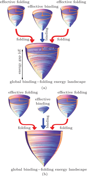
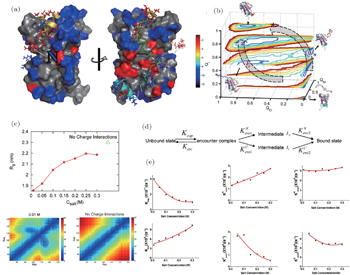

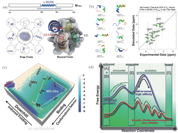
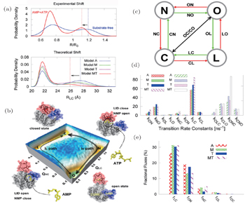


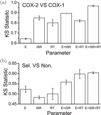
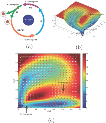
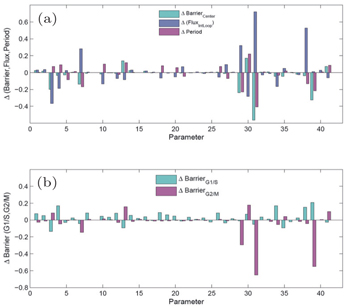

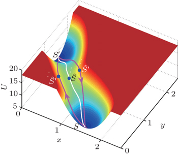
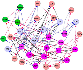

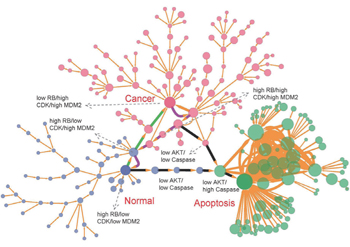
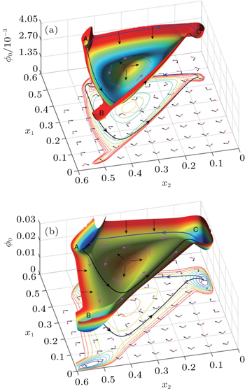
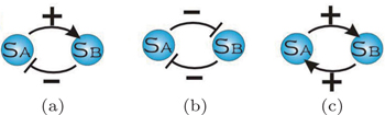


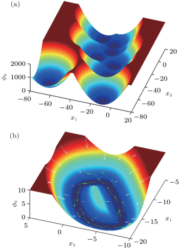
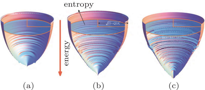


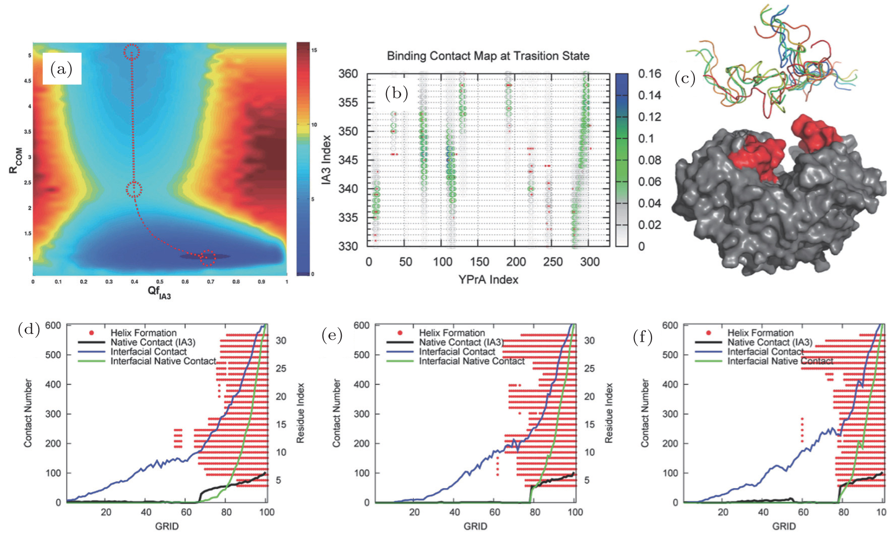
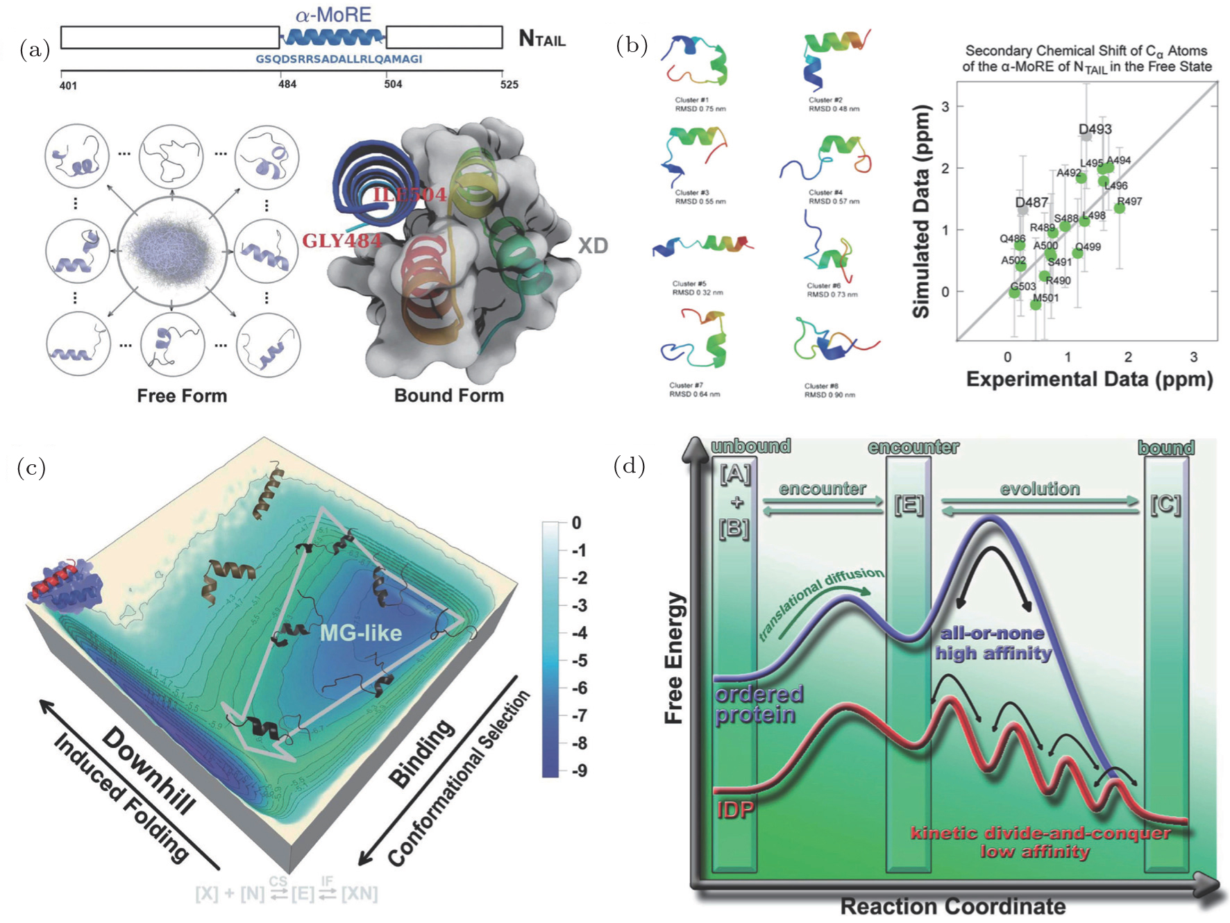

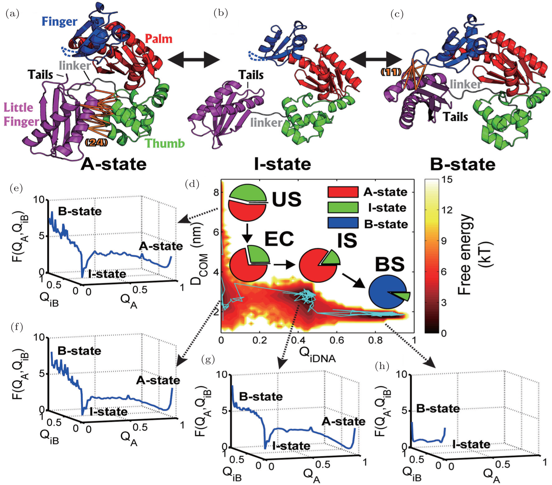
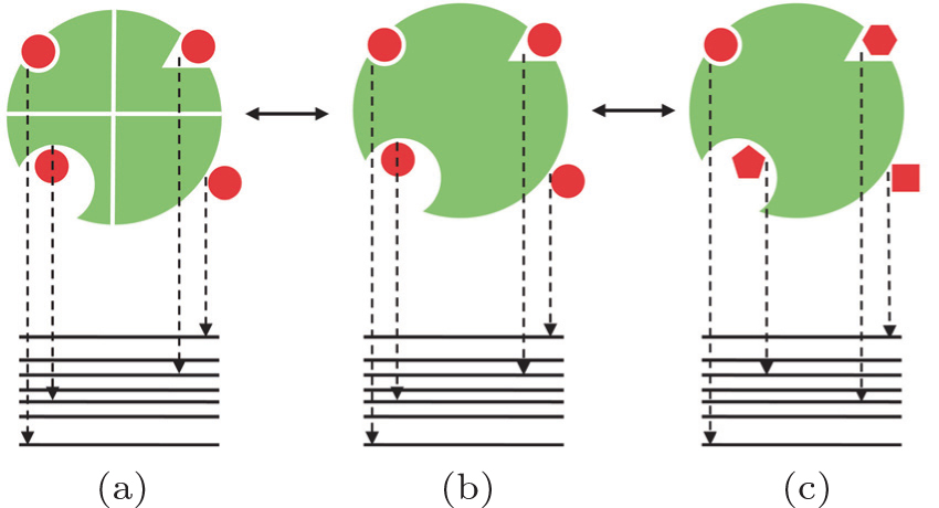
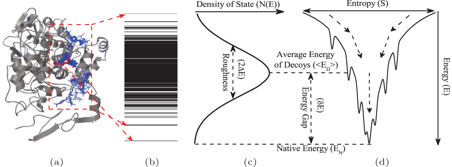
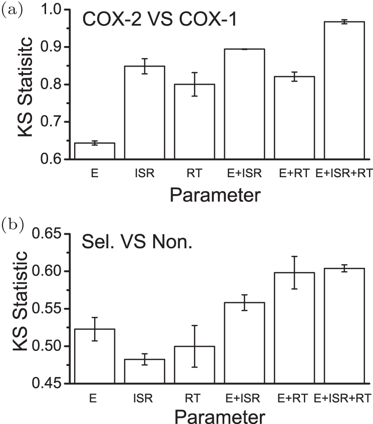


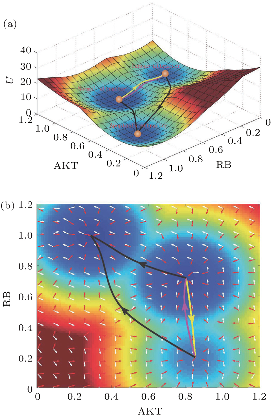


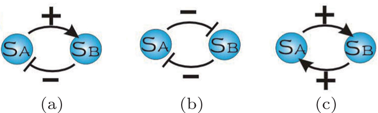
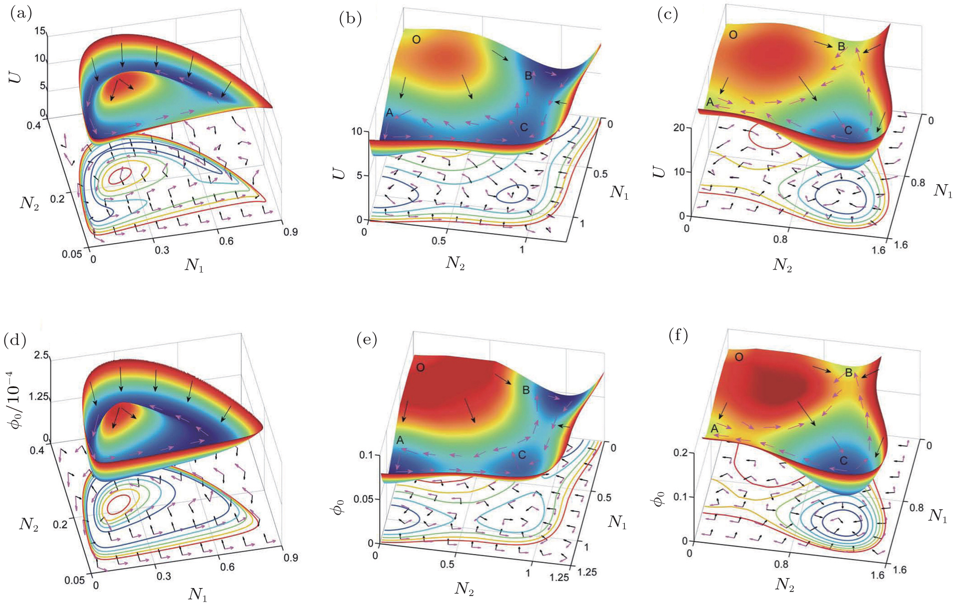
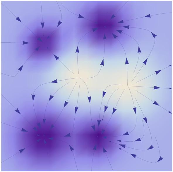

 , Chu Xiakun 1 , Yan Zhiqiang 1 , Zheng Xiliang 1 , Zhang Kun 1 , Zhang Feng 1 , Yan Han 1 , Wu Wei 1 , Wang Jin 1, 2, ‡,