


Three-dimensional multi-relaxation-time lattice Boltzmann front-tracking method for two-phase flow
[Xie Hai-Qiong 1, 2 , Zeng Zhong 1, 2, 3, †,  , Zhang Liang-Qi 1, 2 ]
, Zhang Liang-Qi 1, 2 ]


† Corresponding author. E-mail:
Project supported by the National Natural Science Foundation of China (Grant No. 11572062), the Fundamental Research Funds for the Central Universities, China (Grant No. CDJZR13248801), the Program for Changjiang Scholars and Innovative Research Team in University, China (Grant No. IRT13043), and Key Laboratory of Functional Crystals and Laser Technology, TIPC, Chinese Academy of Sciences.
We developed a three-dimensional multi-relaxation-time lattice Boltzmann method for incompressible and immiscible two-phase flow by coupling with a front-tracking technique. The flow field was simulated by using an Eulerian grid, an adaptive unstructured triangular Lagrangian grid was applied to track explicitly the motion of the two-fluid interface, and an indicator function was introduced to update accurately the fluid properties. The surface tension was computed directly on a triangular Lagrangian grid, and then the surface tension was distributed to the background Eulerian grid. Three benchmarks of two-phase flow, including the Laplace law for a stationary drop, the oscillation of a three-dimensional ellipsoidal drop, and the drop deformation in a shear flow, were simulated to validate the present model.
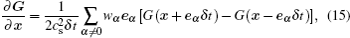
The immiscible two-phase flow with an interface appears immensely in both industrial and natural processes, which drives the development in modeling and simulating the twophase flow. The main difficulty associated with the numerical simulation is modeling the dynamical interface and computing accurately the surface tension. Traditionally, the macroscopic Navier–Stokes (N–S) equations for the two-phase flow are solved together with a proper technique to update the interface location between different phases. There are three commonly used techniques to capture the interface, including the fronttracking method, [ 1 ] the volume of fluid (VOF) method, [ 2 ] and the level set method. [ 3 ] Each method has its own advantages. The front-tracking method represents the interface in a Lagranian fashion and the surface tension is implemented directly at the interface location, thus the front-tracking method captures explicitly the dynamic interface. VOF and level set methods deal naturally the breaking and coalescing interface, and both methods solve an advection equation to capture the interface in an Eulerian grid.
In the above mentioned models for the two-phase flow, the flow field is represented by solving directly the incompressible N–S equations. More recently, the lattice Boltzmann method (LBM) has been developed for computational fluid dynamics (CFD). Different from solving directly the N–S equations (second-order non-linear partial differential equations) in the traditional CFD methods, LBM adopts only a first-order partial differential equation as the evolution equation. In addition, LBM has several advantages over the traditional CFD methods, especially in dealing with complex boundaries, incorporating microscopic interactions, and parallelization of the algorithm. [ 4 ] Recently, LBM has been widely adopted to simulate the two-phase fluid–structure interaction [ 5 – 7 ] and thermal fluid flows. [ 8 , 9 ]
In the LBM framework, several hybrid methods, which incorporate LBM with interface tracking techniques, have been developed. Mehravaran and Hannani, [ 10 , 11 ] Thommes et al. , [ 12 ] and Becker et al. [ 13 ] incorporated LBM with the level set method to simulate the immiscible two-phase flow. In their hybrid method, the flow fields are simulated by LBM with a BGK operator, and the level set method is applied to capture the evolution of the interface between two fluids. Lallemand et al. [ 14 ] proposed a hybrid method, in which the twodimensional flow field is solved by LBM using an Eulerian grid and the interface of two fluids is tracked by using a Lagrangian grid.
Inspired by the hybrid model for the two-phase flow, in this study, we develop a lattice Boltzmann front-tracking method to study the three-dimensional two-phase flow with a sharp dynamical interface based on our previous work for the two-dimensional flow. [ 15 ] The LBM model with a multiplerelaxation- time collision process for better stability is applied to simulate the three-dimensional flow field on an Eulerian grid, an additional Lagrangian grid is adopted to track explicitly the interface motion, and an indicator function is introduced to update the fluid properties. Three verification cases are conducted for both static and dynamical interfaces.
In this section, three basic parts of our hybrid LBM approach are introduced. The flow field is solved by the multirelaxation- time LBM, the front-tracking method is adopted to capture the dynamical interface, and the surface tension is implemented directly on the interface.
The LBM model has three ingredients. The first ingredient is a discrete phase space defined by a regular lattice together with a set of symmetric discrete velocities { 


The transformation matrix
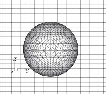
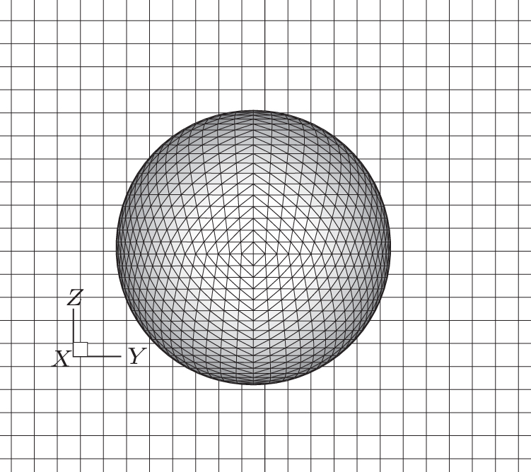
In this work, the D3Q19 model is adopted as shown in Fig.

 | Fig. 1. Illustration of the D3Q19 lattice. |
The equilibrium distribution moments


The nineteen equilibrium distribution moments of this model are


The parameters s 0 , s 3 , s 5 , and s 7 are the relaxation times corresponding to the collision invariants. The parameters s 9 , s 11 , s 13 , and s 15 are related to the kinematic viscosity ν by 

The fluid macroscopic fluctuation density δρ and velocity


When the evolution equation (
 | Fig. 2. The Eulerian grid for flow field and Lagrangian grid for interface. |
The reconstruction of the fluid properties b (


The Poisson equation is solved by a standard second-order centered difference method, and the linear equation is solved with a traditional successive-over-relaxation method. Here


The partial derivatives in Eq. (
This discretization is based on the lattice-based stencil, instead of the standard stencil based on the coordinate directions. A smooth indicator function can be constructed by solving the Poisson equation (
The governing equation ( 


As the interface makers move, the interface grid resolution may change, which has a strong effect on the information exchange between Lagrangian grid and Eulerian grid. Therefore, an adaptive Lagrangian grid is adopted to maintain the resolution during the simulation. In this study, restructuring the Lagrangian grid for the interface consists of two operations, edge split and edge deletion. For a short edge, the edge is removed, and for a long edge, an additional maker is placed in the middle of the edge. Generally, we take the maximum edge length as the Eulerian grid size, and the minimum edge length as 0.3 times the Eulerian grid size.
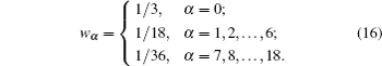
Calculating accurately the surface tension is a great challenge in simulating the two-phase flow. In this study, the surface tension is computed from the tensile forces on the three edges of all interface elements m (see Fig.

 | Fig. 3. The surface tension on element m with three neighboring surface elements. |
In this section, the three-dimensional MRT LBM model incorporating front-tracking technique is validated by three benchmark cases, including the Laplace law for a stationary drop, the oscillation of a three-dimensional ellipsoidal drop, and the drop deformation in a shear flow. Unless otherwise specified, we express the results in lattice units.
Initially, a three-dimensional spherical drop locates at the center of the domain, and a homogenous pressure is set initially. The periodic boundary conditions are imposed at all boundaries. According to the Laplace law, the pressure difference across the drop interface at equilibrium is related to the surface tension

In this numerical computation, we consider four different radii 10, 12, 14, and 16. The corresponding three-dimensional domain is discretized by 6 R × 6 R × 6 R lattice units. In all the cases, the surface tension σ is set to be 0.01, the kinematic viscosity ν is equal to 0.1, and two different density ratios are adopted. Table 
| Table 1. Pressure differences across the interface for different drop radii from LBM simulations and the theoretical solution based on the Laplace law. . |
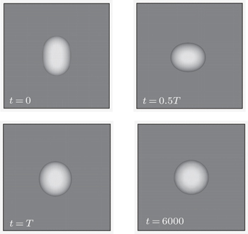
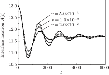
The oscillation of a three-dimensional ellipsoidal drop, which immerses in another fluid, is considered. The frequency of the oscillatory drop is given in Ref. [ 20 ]


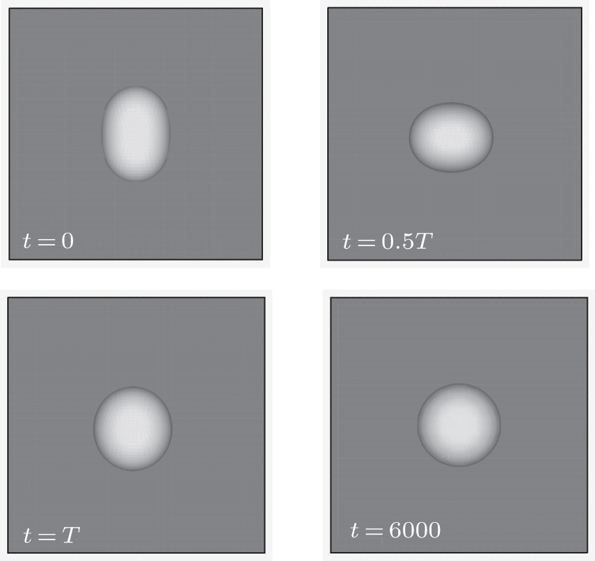 | Fig. 4. Configurations of an oscillating drop at different time. |
Initially, the minimum and the maximum radii of the ellipsoidal drop are 11 and 13, respectively. The ellipsoidal drop is placed in the domain center, and the domain is 72 × 72 × 72 lattice units. Table
| Table 2. Comparison of the oscillation periods between the analytical solutions and the LBM results for different viscosities. . |
 | Fig. 5. Interface location of an oscillating drop as a function of time for different kinematic viscosities. |
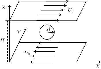
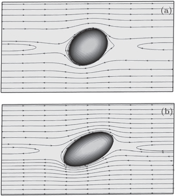
In this section, a three-dimensional numerical simulation is performed on the classical Taylor experiment, the drop deformation within a shear flow as illustrated in Fig.


 | Fig. 6. Drop deformation within a shear flow. |
The parameters are adopted as ρ i = ρ o = 1, σ = 0.01, Re = 0.1, and the viscosity of the drop is equal to the surrounding fluid. The capillary number varies from 0.05 to 0.30. The computational domain is 12 R × 6 R × 6 R lattice units. Figure
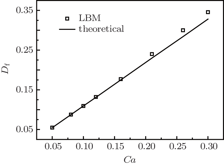 | Fig. 7. Taylor deformation parameter D f as a function of the capillary number at Re = 0.1. |
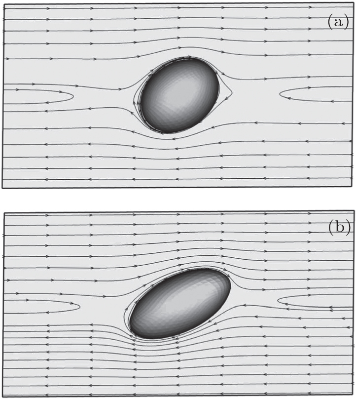 | Fig. 8. Velocity field in the x – z plane and the deformed droplet: (a) Ca = 0.1, (b) Ca = 0.26. |
We have developed an MRT lattice Boltzmann model incorporating the front-tracking technique to simulate the twophase flow with a dynamical interface. The flow field was simulated by LBM method on an Eulerian grid, and an adaptive unstructured triangular Lagrangian grid was applied to track explicitly the interface motion. Three benchmark cases were simulated to validate this model. In the benchmark of a threedimensional spherical drop, the Laplace law is well satisfied with the simulated pressure difference across the interface. In the benchmark of an oscillating ellipsoidal drop, the simulated oscillatory period is consistent with the theoretical solution. In the benchmark of the drop deformation in a shear flow, the simulated drop deformation coincides well with the theoretical solution for small capillary number.
| 1 | |
| 2 | |
| 3 | |
| 4 | |
| 5 | |
| 6 | |
| 7 | |
| 8 | |
| 9 | |
| 10 | |
| 11 | |
| 12 | |
| 13 | |
| 14 | |
| 15 | |
| 16 | |
| 17 | |
| 18 | |
| 19 | |
| 20 | |
| 21 |