The researchers at present are engaged in exploring the flows of non-Newtonian fluids at various aspects. Non- Newtonian fluids are very popular due to their importance in our daily life. Examples of such fluids include sugar solutions, apple sauce, lubricants, shampoos, cosmetic products, tomato ketchup, and many others. There is no single constitutive relation describing the characteristics of all non-Newtonian fluids. The simplest subclass of the rate-type fluid is the Maxwell fluid. It only predicts the stress relaxation effects but not the stress retardation effects. Owing to such a disadvantage, an Oldroyd-B fluid model was proposed to investigate both stress relaxation and retardation effects. This model was studied in the past by various investigators under different flow geometries and physical aspects. Some studies on flows of an Oldroyd-B fluid can be found in Refs. [ 1 ]–[ 7 ]. Besides these, Shivakumara and Sureshkumar ^{[ 8 ]} reported the effects of flow and quadratic drag on the stability of an Oldroyd-B fluid in a porous space. Khan and Zeeshan ^{[ 9 ]} addressed the electrically conducting flow of an Oldroyd-B fluid induced by sawtooth pulses. Liu et al . ^{[ 10 ]} analyzed the unsteady Couette flow of an Oldroyd-B fluid with fractional derivative. The authors reported the solutions through the Laplace transform method. Swamy and Sidram ^{[ 11 ]} discussed the effect of rotation on the thermal convection flow of an Oldroyd-B fluid. The influences of viscoelastic parameters in the thermal convection flow of an Oldroyd-B fluid with constant heat flux were discussed by Niu et al. ^{[ 12 ]} Shivakumara et al. ^{[ 13 ]} addressed the thermal convection instability of an Oldroyd-B fluid saturating through a porous medium. The steady stagnation point flow of an Oldroyd-B fluid with mixed convection was numerically analyzed by Sajid et al . ^{[ 14 ]}

The dynamics of heat transfer phenomenon is a subject of special attention due to its abundant applications in engineering and industrial processes. Examples of such applications include wire drawing, cooper materials, nuclear reactor cooling, heat conduction in tissues, refrigeration, heat pumps, energy production, cooling of electronic devices, etc. The Fourier’s law of heat conduction ^{[ 15 ]} explores the characteristics of heat transfer mechanism at various aspects. The main disadvantage of this model is that it leads to a parabolic energy equation which indicates that the initial disturbance is instantly experienced by the medium under observation. To overcome this disadvantage, Cattaneo ^{[ 16 ]} presented the modified Fourier’s law of heat conduction by introducing a relaxation time term. The frame-indifferent generalization of Cattaneo’s law through the implementation of Oldroyds’ upper convective derivative was developed by Christov. ^{[ 17 ]} Ostoja-Starzewski ^{[ 18 ]} gave the mathematical derivation of the Maxwell–Cattaneo equation by involving a material time derivative of heat flux. The stability and uniqueness of the solutions constructed by the Cattaneo–Christov heat flux model were discussed by Tibullo and Zampoli. ^{[ 19 ]} The numerical solutions of an incompressible thermal convection fluid with the Cattaneo–Christov model were constructed by Straughan ^{[ 20 ]} and Haddad. ^{[ 21 ]} The structural stability and uniqueness of the Cattaneo–Christov heat flux equations were reported by Ciarletta and Straughan. ^{[ 22 ]} Al-Qahtani and Yilbas ^{[ 23 ]} provided the closed form solutions of Cattaneo and stress equations via the Laplace transform method. Papanicolaou et al. ^{[ 24 ]} investigated the influence of the thermal relaxation time in the Cattaneo–Maxwell equations subjected to vertical and horizontal temperature gradients. Very recently, Han et al . ^{[ 25 ]} considered the Cattaneo–Christov heat flux model for a boundary layer flow of Maxwell fluid over a stretching sheet. The authors developed the homotopic solutions. Mustafa ^{[ 26 ]} reported the numerical and homotopic solutions for a two-dimensional flow of Maxwell fluid in a rotating frame. Bissell ^{[ 27 ]} discussed an oscillatory convection flow with the Cattaneo–Christov hyperbolic heat model.

In the present analysis, we introduce the Cattaneo– Christov heat flux model for a two-dimensional boundary layer flow of an Oldroyd-B fluid over a stretching sheet. An incompressible laminar fluid is taken into account. The governing nonlinear ordinary differential equations are solved by the optimal homotopy analysis method (OHAM). ^{[ 28 – 33 ]} Convergent series solutions are developed. Graphical results of dimensionless velocity and temperature fields are sketched and examined.

We consider a two-dimensional boundary layer flow of an incompressible Oldroyd-B fluid over a linearly stretching sheet. The laws of conservation of mass and momentum for the incompressible fluid are

The Cattaneo–Christov heat flux model can be written as ^{[ 17 , 19 ]}

The energy equation for the steady incompressible boundary layer flow is

The temperature equation governing the steady-state laminar flow is

The associated boundary conditions for the temperature are

In the above equations, α is the thermal diffusivity, T _w is the temperature at the wall, and T _∞ is the ambient fluid temperature.

Equations ( 2 ), ( 3 ), ( 6 ), and ( 7 ) can be reduced into the dimensionless form by introducing the following new variables:

The equations of momentum, energy, and concentration in dimensionless form are

We solve Eqs. ( 9 ) and ( 10 ) with the boundary conditions ( 11 ) and ( 12 ) through the optimal homotopy analysis approach. Keeping in view the so-called rule of solution expression and the boundary conditions ( 9 ) and ( 10 ), it is appropriate to select the following set of base functions: ^{[ 34 ]}

We can express f ( η ) and θ ( η ) in the following forms: ^{[ 35 , 36 ]}

The above initial guess and auxiliary linear operators satisfy the following properties:

3.2. The m -th order deformation problems

The m -th order problems can be constructed as follows:

The general solutions can be written as

where and are the special solutions. The constants C ₁ – C ₅ are given by

The squared residuals of the governing equations are defined in the following forms:

Such a kind of error is considered in various recent papers. ^{[ 29 – 33 ]} The best possible values of ℏ at a given order of approximation may be computed by minimizing the squared residuals E _{f , M} and E _{θ , M} . This can be achieved through the command Minimize of the software Mathematica (see Ref. [ 28 ] for details). The optimal values of ℏ for the functions f and θ are given in Tables 1 and 2 .

Table 1.

Table 1.

Table 1. Optimal auxiliary parameter ℏ for function f at the 15th order approximation for different β 1 when β 2 = 0.5. . β 1 Optimal ℏ Minimum E f , M 0 −0.768 4.32× 10 −22 0.25 −0.504 1.54× 10 −11 0.50 −0.565 2.38× 10 −11 0.75 −0.583 3.86× 10 −11 1.00 −0.560 4.27× 10 −10

Table 1. Optimal auxiliary parameter ℏ for function f at the 15th order approximation for different β 1 when β 2 = 0.5. .

Table 2.

Table 2.

Table 2. Optimal auxiliary parameter ℏ for function θ at 15th order approximation for different γ when β 2 = 0.5. . γ Optimal ℏ Minimum E θ , M 0 −0.903 8.86× 10 −12 0.25 −0.926 1.84× 10 −9 0.50 −0.987 8.62× 10 −8 0.75 −0.978 1.38× 10 −6 1.00 −0.511 2× 10 −4

Table 2. Optimal auxiliary parameter ℏ for function θ at 15th order approximation for different γ when β 2 = 0.5. .

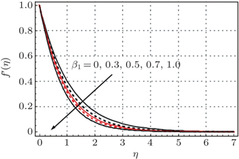
Figures 1 and 2 are drawn to examine the influences of Deborah numbers β ₁ and β ₂ on the dimensionless velocity field f ′( η ). From Fig. 1 , we find that the velocity field and the momentum boundary layer thickness are decreasing functions of Deborah number β ₁ . The Deborah number β ₁ appears due to the relaxation time. The larger Deborah number β ₁ corresponds to longer relaxation time and such longer relaxation time resists the fluid flow due to lower velocity and thinner momentum boundary layer. On the other hand, an increase in the Deborah number β ₂ gives an enhancement to the velocity field and the momentum boundary layer thickness (see Fig. 2 ). In fact, the Deborah number β ₂ is directly related to the retardation time and the retardation time has an ability to enhance the fluid velocity. Here the Maxwell fluid flow case is obtained by setting β ₂ = 0. Moreover, the viscous fluid case is obtained when β ₁ = 0 = β ₂ .

Fig. 1.

	Figure Option View Download New Window
	Fig. 1. Variation of dimensionless velocity field f ′( η ) with η for different β 1 when β 2 = 0.2.

Fig. 2.

	Figure Option View Download New Window
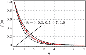
	Fig. 2. Variation of dimensionless velocity field f ′( η ) with η for different β 2 when β 1 = 0.4.

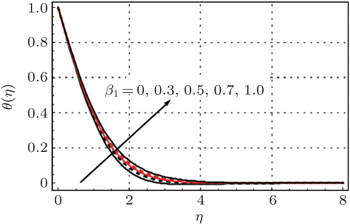
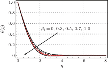
The variations in dimensionless temperature profile θ ( η ) corresponding to different Deborah numbers β ₁ and β ₂ , Deborah number γ with respect to the heat flux relaxation time and Prandtl number Pr are shown in Figs. 3 – 6 . From Figs. 3 and 4 , we note that the Deborah numbers β ₁ and β ₂ have quite reverse effects on the temperature profile and the thermal boundary layer thickness. The temperature profile is enhanced with the increase of the Deborah number β ₁ , but it reduces for larger Deborah number β ₂ . Physically, the Deborah numbers β ₁ and β ₂ appear due to the relaxation time and the retardation time, respectively, and these parameters have quite opposite effects on the temperature and the heat transfer rate. The involvements with the relaxation time and the retardation time here are responsible for the reduction and enhancement of the temperature profile and the thermal boundary layer thickness. Figure 5 shows that the temperature profile and the thermal boundary layer thickness are lower for larger Deborah number γ . The Deborah number γ arises due to the heat flux relaxation time. The fluid with longer heat flux relaxation time has lower temperature, and the fluid with shorter heat flux relaxation time corresponds to higher temperature. Here the longer heat flux relaxation time is obtained when we increase the Deborah number γ . Such longer heat flux relaxation time corresponds to higher heat transfer rate and smaller temperature due to the reduction in temperature and thermal boundary layer thickness. The Cattaneo–Christov heat flux model is reduced to simple Fourier’s law of heat conduction when γ = 0. The effects of the Prandtl number on the temperature profile are explored in Fig. 6 . It is observed that an increase in the Prandtl number leads to a reduction in the temperature and thermal boundary layer thickness. The Prandtl number is the ratio of momentum to thermal diffusivity. The thermal diffusivity is weaker for larger Prandtl number due to the fact that the rate of diffusion decreases. Such a reduction in the diffusion rate acts as an agent showing a reduction in the temperature and thermal boundary layer thickness. The suitable Prandtl numbers are quite essential in the industrial processes, because they are used to control the heat transfer rate during the final product.

Fig. 3.

	Figure Option View Download New Window
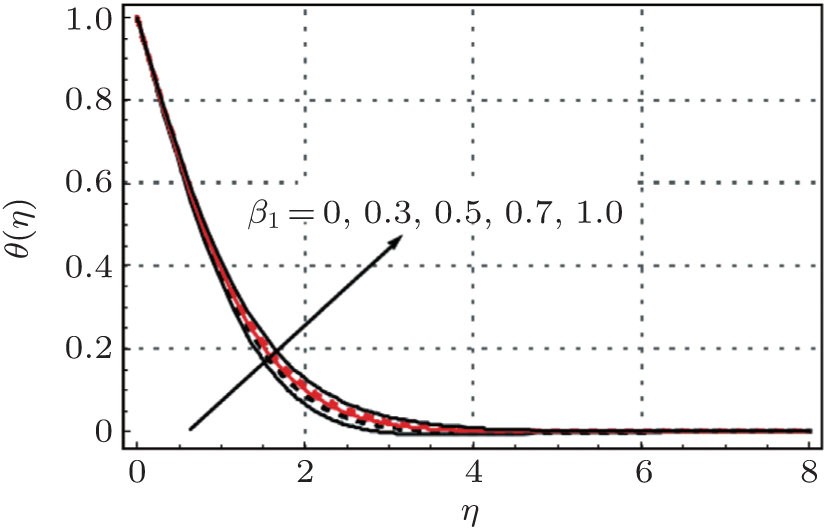	Fig. 3. Variation of dimensionless temperature field θ ( η ) with η for different β 1 when β 2 = 0.2, γ = 0.3, and Pr = 1.4.

Fig. 4.

	Figure Option View Download New Window
	Fig. 4. Variation of dimensionless temperature field θ ( η ) with η for different β 2 when β 1 = 0.4, γ = 0.3, and Pr = 1.4.

Fig. 5.

	Figure Option View Download New Window
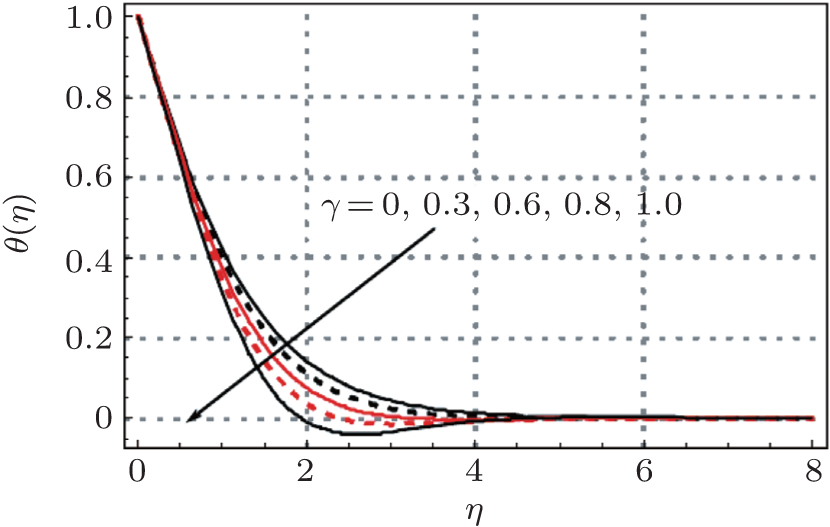	Fig. 5. Variation of dimensionless temperature field θ ( η ) with η for different γ when β 1 = 0.4, β 2 = 0.2, and Pr = 1.

Tables 1 and 2 present the optimal values of convergence control parameters at the 15th order of deformations for various values of β ₁ and γ . Table 3 is for comparison with the numerical solutions obtained by Abel et al . ^{[ 39 ]} and Megahed ^{[ 40 ]} in the limiting case for different Deborah numbers β ₁ . From this table, we notice that our series solutions are in excellent agreement with the numerical solutions provided by Abel et al . ^{[ 39 ]} and Megahed. ^{[ 40 ]} Table 4 shows the comparative values of f ″(0) for various values of β ₁ given by Sadghey et al . ^{[ 41 ]} and Mukhopadhyay. ^{[ 42 ]} This table also clearly indicates that our present analytical solutions are in very good agreement with the solutions of Sadghey et al . ^{[ 41 ]} and Mukhopadhyay ^{[ 42 ]} in the limiting case. It is also observed that the values of f ″(0) are larger for higher values of β ₁ . The Deborah number β ₁ is directly proportional to the relaxation time λ ₁ . The λ ₁ is increased for larger β ₁ . Such longer relaxation time reduces the fluid velocity but enhances f ″(0). Table 5 shows the numerical values of f ″(0) for different Deborah numbers β ₂ when β ₁ = 0.4. This table clearly presents that f ″(0) is reduced as Deborah number β ₂ increases. The retardation time λ ₂ is involved in β ₂ which is enhanced for larger β ₂ . Such an enhancement in retardation leads to a reduction in f ″(0). Table 6 is for examining the temperature gradient θ ′(0) for different β ₂ , Pr , and γ when β ₁ = 0.5. Here we can see that an increase in β ₂ gives rise to larger temperature gradient θ ′(0). The temperature gradient θ ′(0) increases for larger Pr but decreases for larger γ . The Prandtl number strongly depends on the thermal diffusivity of fluid, and the larger Prandtl number corresponds to weaker thermal diffusivity due to the fact that the temperature gradient is increased.

Fig. 6.

	Figure Option View Download New Window
	Fig. 6. Variation of dimensionless temperature field θ ( η ) with η for different Pr when β 1 = 0.4, β 2 = 0.2, and γ = 0.3.

Table 3.

Table 3.

Table 3. Comparison with f ″(0) obtained by Abel et al . [ 39 ] and Megahed [ 40 ] for different β 1 when β 2 = 0. . β 1 Abel et al. Megahed Present results 0.0 0.999962 0.999978 1.00000 0.2 1.051948 1.051945 1.05189 0.4 1.101850 1.101848 1.10190 0.6 1.150163 1.150160 1.15014 0.8 1.196692 1.196690 1.19671 1.2 1.285257 1.285253 1.28536 1.6 1.368641 1.368641 1.36873 2.0 1.447617 1.447616 1.44781

Table 3. Comparison with f ″(0) obtained by Abel et al . [ 39 ] and Megahed [ 40 ] for different β 1 when β 2 = 0. .

Table 4.

Table 4.

Table 4. Comparison with f ″(0) obtained by Sadghey et al . [ 41 ] and Mukhopadhyay [ 42 ] in the limiting case for different β 1 by fixing β 2 = 0. . β Sadghey et al . Mukhopadhyay Present solutions 0.0 1.0000 0.9999963 1.00000 0.2 1.0549 1.051949 1.05189 0.4 1.10084 1.101851 1.10190 0.6 1.0015016 1.150162 1.15014 0.8 1.19872 1.196693 1.19671

Table 4. Comparison with f ″(0) obtained by Sadghey et al . [ 41 ] and Mukhopadhyay [ 42 ] in the limiting case for different β 1 by fixing β 2 = 0. .

Table 5.

Table 5.

Table 5. Values of f ″(0) for different β 2 when β 1 = 0.4. . β 2 − f ″(0) 0.0 1.10190 0.2 1.00498 0.4 0.92986 0.6 0.86942 0.8 0.81943 1.0 0.77718

Table 5. Values of f ″(0) for different β 2 when β 1 = 0.4. .

Table 6.

Table 6.

Table 6. Values of − θ ′(0) for different β 2 , Pr , and γ when β 1 = 0.5. . β 2 Pr γ − θ ′(0) 0.0 1.0 0.3 0.56621 0.2 1.0 0.3 0.58970 0.5 1.0 0.3 0.61671 0.3 0.8 0.3 0.51088 0.3 1.2 0.3 0.68070 0.3 1.6 0.3 0.82621 0.3 1.0 0.0 0.57276 0.3 1.0 0.2 0.59032 0.3 1.0 0.5 0.61927

Table 6. Values of − θ ′(0) for different β 2 , Pr , and γ when β 1 = 0.5. .

We explore the properties of the Cattaneo–Christov heat flux model for a two-dimensional hydrodynamic boundary layer flow of an Oldroyd-B fluid over a stretching sheet. The obtained key features are listed below.

•

The velocity field decreases while the temperature profile increases as the Deborah number β ₁ increases.