Ab initio path-integral molecular dynamics and the quantum nature of hydrogen bonds
[Feng Yexin 1 , Chen Ji 1 , Li Xin-Zheng 2, 3, †,  , Wang Enge 1, 3 ]
, Wang Enge 1, 3 ]
|
|


† Corresponding author. E-mail:
Project supported by the National Natural Science Foundation of China (Grant Nos. 11275008, 91021007, and 10974012) and the China Postdoctoral Science Foundation (Grant No. 2014M550005).
The hydrogen bond (HB) is an important type of intermolecular interaction, which is generally weak, ubiquitous, and essential to life on earth. The small mass of hydrogen means that many properties of HBs are quantum mechanical in nature. In recent years, because of the development of computer simulation methods and computational power, the influence of nuclear quantum effects (NQEs) on the structural and energetic properties of some hydrogen bonded systems has been intensively studied. Here, we present a review of these studies by focussing on the explanation of the principles underlying the simulation methods, i.e., the ab initio path-integral molecular dynamics. Its extension in combination with the thermodynamic integration method for the calculation of free energies will also be introduced. We use two examples to show how this influence of NQEs in realistic systems is simulated in practice.
The hydrogen bond (HB) is a generally weak but ubiquitous intermolecular interaction. It is responsible, for example, for holding together the two strands of DNA molecules and many phases of water. As such, understanding the behaviors of HBs is lying at the core of many studies concerning the behaviors of water and biomolecules. The small mass of hydrogen (H) means that many of these problems are quantum mechanical in nature, [ 1 – 7 ] although all too often these nuclear quantum effects (NQEs) are neglected. These NQEs are essential for rationalizing many phenomena of te H-bonded systems, especially where quantum tunneling and zero-point motion are concerned. For example, starting from the 1950s, it has been known that replacing H by deuterium (D) in H-bonded molecular crystals with electronic structures unchanged can result in obvious variations of the lattice constants. [ 8 ] This is currently known as the Ubbelohde effect. [ 9 ] In enzyme reactions, the proton tunneling along HBs is referred to as “nature’s subway”. By using a neutron Compton scattering experiment, a picture concerning the impact of NQEs on the real space delocalization and vibrational properties of the proton in liquid water was also revealed. [ 10 , 11 ] Most recently, a cryogenic scanning tunneling microscope (STM) experiment even confirmed the isotope-dependent switching rate of water tetramer on salt between its two chirality states, which could only be rationalized by considering the NQEs. [ 12 ]
From the theoretical perspective, accurate computer simulations of these phenomena require an accurate quantum mechanical description of the finite-temperature nuclear fluctuations in real polyatomic systems. A natural choice is to construct a high-dimensional Schrödinger equation for the many-body entity of the nuclei. By solving the eigenstate wave-functions of this Schrödinger equation, one can observe not only the statistical but also the dynamical properties of the system under investigation related to the quantum nature of the nuclei. Over the last ∼ 20 years, this method has been extremely successful in describing gas-phase reactions. [ 13 – 17 ] However, because of the notorious scaling problem in mapping the high-dimensional potential energy surface (PES) and solving the Schrödinger equation, the application of this method has been seriously limited to systems with less than ∼ 6 atoms. For more realistic polyatomic systems and condensed matters, a practical method is highly desired. Thanks to the development of the path-integral representation of quantum mechanics starting from the late 1940s, [ 18 – 21 ] a scheme practical for large polyatomic systems and condensed matters in which not only the thermal effects but also the NQEs can be accounted for statistically has been systematically presented by Feynman and Hibbs. [ 22 ] Based on such a foundation, the molecular dynamics (MD) simulation technique was combined with this path-integral representation of quantum mechanics, and a series of path-integral molecular dynamics (PIMD) simulations were carried out in the 1980s, as reported by Chandler, Parrinello, and Berne et al. in Refs. [ 23 ]–[ 25 ], respectively. Analogous to these MD based simulations, the Monte–Carlo (MC) sampling technique can also be used. At roughly the same time, the properties of liquid helium, including its superfluidity, were systematically studied by Ceperley and Pollock using path-integral Monte–Carlo (PIMC) simulations. [ 26 – 29 ] In these PIMD/PIMC simulations, the NQEs are accounted for on the same footing as the thermal effects when the statistical properties are evaluated, as will be explained later in Section 2. Therefore, when comparing their results with the ones obtained in the MD simulations, in which the nuclei are treated classically, the NQEs can be addressed in a very clean manner.
These comparisons set up a rigorous framework for the NQEs to be investigated statistically, which is still used nowadays. However, in these early PIMD and PIMC simulations, researches often resorted to empirical potentials for descriptions of the interatomic interactions. When chemical reactions occur, e.g., a proton transfers along a HB, such a simple parametrization of the interatomic interactions may easily fail. To cope with these problems, in which the impact of the NQEs is usually more interesting, an effort toward combining the ab initio electronic structure calculations with the PIMD/PIMC sampling techniques has been made since the mid 1990s, first within the framework of Car–Parrinello (CP) MD (see e.g., Tuckerman, Marx, and Parrinello et al. ’s work in Refs. [ 1 ], [ 30 ], and [ 31 ]) and later by directly using Born–Oppenheimer (BO) MD/MC. [ 6 , 7 , 32 – 34 ] These methods allow for bond making and breaking events, as well as the thermal and quantum nuclear fluctuations to be addressed in a seamless manner based on the forces computed “on-the-fly” as the system evolves, therefore making PIMD/PIMC simulations for problems with complicated chemical environments possible. Currently, not only different functionals within the density-functional theory (DFT) [ 35 – 37 ] but also many traditional quantum chemistry methods such as MP2 [ 38 , 39 ] can be used in descriptions of the electronic structures and consequently the interatomic interactions. With such a wide range of choices for the electronic structures, one can safely rely on the results obtained from such simulations, if the accuracy of the interatomic interaction description and the sampling sufficiency are ensured. We note, however, that such an ensurance is far from being trivial. [ 30 , 35 , 36 ]
The above-mentioned recipe allows the NQEs to be described in a clean manner, if the molecular simulation time is long enough to address the issue of interest. A common problem for most molecular simulation techniques, however, is that the timescale one can afford is not long enough to allow the system to travel between different stable states, thereby hindering a direct evaluation of the free-energy differences between different meta-stable states. In such cases, to determine the relative stability of these different meta-stable states without resorting to the coarse-grained models, [ 40 ] the method one often chooses is to enhance the sampling efficiency either by imposing constraints or modifying the effective PES. [ 41 – 44 ] However, if it is the case that within the molecular simulation time, the system can stay within the local minima of the PES with all spatial configurations close to it explored, a comparison of the free energies associated with each local minimum directly without requiring the system to travel between different meta-stable states provides an alternative. In such cases, a method with which the free energy of each meta-stable state can be calculated is highly desired. When the influence of NQEs on these free energies needs to be quantified, a combination between the thermodynamic integration (TI) method and PIMD is a natural choice. [ 45 , 46 ] In the following, in addition to a general introduction to ab initio PIMD and its application to the studies of some H-bonded systems, a combination of the TI method with ab initio PIMD along with applications of this method to the free-energy calculations of some H-bonded systems will also be discussed.
The paper is organized as follows. An introduction to the ab initio PIMD method and its combination with TI, as well as the computational setups, are given in Section 2. In Section 3, we take a basic question in physics and chemistry, i.e., what is the impact of NQEs on the strength of HB, as an example to show how the ab initio PIMD method can be used to study such problems in H-bonded systems. As the second example, we quantitatively analyze the influence of NQEs on the free energy of some gas phase water clusters using a combination of ab initio PIMD and TI methods in Section 4. Conclusions and a short perspective are given in Section 5.
Using the electronic structures and consequently the interatomic interactions calculated “on-the-fly”, the basic idea of the ab initio PIMD method is to treat the parameter β = 1/( k B T ) associated with a finite temperature T as an imaginary time and represent quantum mechanically the density matrix of the nuclei at this finite T with an artificial polymer, through


In Eq. (


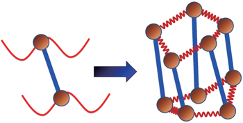
 | Fig. 1. Illustration of how the mapping from the canonical quantum system to a classical polymer is done in the path-integral statistical mechanics. The polymer is composed of P replicas of the real molecule. In each replica, the potential is determined by the potential of the system at the specific spatial configuration of this replica. In between the replicas, the neighboring images (beads) of the same atoms are linked by springs. The spring constant is determined by m j and ω P as   |
Using the method described above, by comparing the results obtained from the ab initio MD and the ab initio PIMD simulations, the influence of NQEs can be analyzed in a very clean manner. However, as mentioned, the molecular simulation time needs to be sufficiently long to address the problem we are interested in. When the timescale one can afford is not long enough to allow the system to travel between different meta-stable states, direct evaluation of the free-energy differences between them becomes technically difficult. One method that is often chosen is to enhance the sampling efficiency either by imposing constraints or modifying the effective PES. [ 41 – 44 ] But as said, if it is the case that within the molecular simulation time, the system stays within each meta-stable state with all spatial configurations close to it explored, a comparison of the free energies of the meta-stable states without requiring the system to travel between them provides an alternative. In this case, one needs a method with which the free energy associated with each local minimum can be calculated. Here, we choose the TI method for such calculations.
The basic idea behind the TI method is that a system with unknown free energy, which we call the reference system, can be connected to a system with known free energy, which we call the real system, by varying one or more parameters. There are several choices for the reference system and the real system, depending on which property we are investigating. In the present work, we want to investigate the influence of NQEs on the free energy of the polyatomic system. Therefore, we have chosen the reference system as the one with classical nuclei, and the real system as the one with quantum nuclei. For the real system, the partition function follows Eqs. (


In between the reference system whose effective potential is given by Eq. (


Two separate works will be reviewed in this manuscript, i.e., (i) the investigation of the influence of NQEs on the structural change of some H-bonded systems, and (ii) the influence of NQEs on the free energy of some water clusters. They were carried out using different codes. But in both of them, the Perdew–Burke–Ernzerhof (PBE) functional was used in the description of the electronic exchange–correlation interactions. [ 53 ] In the following, we summarize their other computational details one after the other.
For investigation of the impact of NQEs on the HB strength (using the geometric property changes as an indicator), the simulations were carried out using the CASTEP plane-wave density-functional theory (DFT) code. [ 54 ] The ultrasoft pesudopotentials were taken along with a 400 eV energy cutoff for the expansion of the wavefunction. For simulation of the water and HF clusters, a 12 Å cubic cell was used. For the organic dimers and charged water clusters, an 18 Å cubic cell was taken. For solid HF and HCl, an eight molecule supercell along with a 4 × 2 × 3 Monkhorst–Pack k -point mesh was used. For the solid squaric acid, a 20-atom cell along with a 3 × 3 × 2 Monkhorst–Pack k -point mesh was chosen. Time steps of 0.5–0.7 fs were used, and after thermalization, 10000 MD and 6000 PIMD steps were performed. All the MD and PIMD simulations reported for this part of the work were performed at a targeting temperature of 100 K, except in solid HCl 
For the free-energy change due to NQEs in water clusters, a self-developed combination of the TI and the ab initio PIMD method within the Vienna ab initio simulation package (VASP) was used. [ 56 , 57 ] Projector-augmented wave potentials were employed along with a 600 eV plane wave cutoff energy for the expansion of the Kohn–Sham orbitals. The Andersen thermostat was used to control the temperature of the NVT ensemble. [ 58 ] The temperature was set as 100 K, safely with the stability of the clusters. 48 beads were used to sample the imaginary time path-integral with a time step of 0.5 fs. After thermalization, 30000 PIMD steps were used at each λ along the TI line to obtain the F ′( λ ). For more computational details, please refer to Ref. [ 57 ].
The first example of the ab initio PIMD simulations, in which the quantum nature of the nuclei plays an important role, concerns a fundamental question in physics and chemistry, i.e., what is the influence of NQEs on the strength of HBs? We start by using the structural properties, namely, the heavy-atom distances, as an indicator. Further investigations on the energetics will be discussed in Section 4. As mentioned earlier in this manuscript, it has been known for more than half a century that, in H-bonded molecular crystals, by replacing H with D, the strength of HBs and consequently the crystal structural parameters change. This phenomenon is known as the Ubbelohde effect. [ 8 , 9 ] The conventional Ubbelohde effect reflects an increase of the heavy-atom distance associated with the HB upon replacing H by D, which indicates that NQEs strengthen this intermolecular interaction. We note, however, that a negative Ubbelohde effect in which a decrease of the heavy-atom distance happens upon replacing H by D has also been observed in several materials. [ 8 , 9 ] From the perspective of molecular simulation, since the 1980s, when PIMD/PIMC becomes a conventional routine to investigate the NQEs in real polyatomic systems, a bunch of computer simulations have been carried out in a wide range of systems. A general conclusion is that the final effect is system-dependent. For example, in liquid HF, ab initio MD and PIMD simulations have shown that when NQEs are accounted for, the first peak of the F–F radial distribution function (RDF) sharpens and shifts to a shorter F–F distance, [ 59 ] indicating that NQEs strengthen the HB in this system. In contrast, a similar simulation for liquid water shows that the O–O RDF gets less structured when NQEs are included, indicating that NQEs weaken the HB in liquid water. [ 2 ] We note, however, that although this conclusion is probably right, it is the opposite of what has been reported in Ref. [ 5 ].
Besides this discussion concerning HBs in condensed phases, the impact of NQEs on the strength of HBs has also been widely discussed in gas-phase clusters. [ 59 – 61 ] For water clusters up to the hexamer, it was predicted that the NQEs weaken the HBs, as reflected by the change of the heavy-atom distances in Refs. [ 60 ] and [ 61 ]. For HF clusters, however, it was predicted that NQEs can strengthen or weaken the HBs depending on the size of the clusters. [ 59 ] For clusters smaller than tetramer, the NQEs weaken this intermolecular interaction, whereas for clusters larger than it, the strengthening of the HB is observed. In tetramer, the NQEs are negligible. With these system-dependent conclusions in mind, it is clear that a simple picture in which the influence of the NQEs on the strength of HBs and consequently the structural or energetic properties can be rationalized is highly desired. In Ref. [ 7 ], we have presented a simple picture which can be used to rationalize these different results. Ab initio PIMD simulations were used as the basic tool upon which the analysis was carried out. Here, using these simulations as an example, we will review this work in a way that how the ab initio MD and PIMD simulations are used to answer this question can be understood in a easy manner.
To be as unbiased as possible, a wide range of H-bonded systems have been chosen, including HF clusters (dimer to hexamer), H 2 O clusters (dimer, pentamer, and octamer), charged, protonated, and hydroxylated water and ammonia clusters ( 


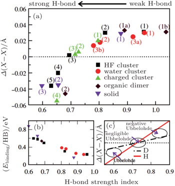
 | Fig. 2. (a) The differences between the shortest heavy-atom distances obtained from the PIMD and MD simulations      |
With the definition of the above-mentioned quantities in mind, we first look at the results for the impact of the NQEs on the strength of HBs. Upon comparing these results for the various H-bonded systems, an interesting correlation can be observed between the H-bond strength and the change in intermolecular separations, as shown in Fig.
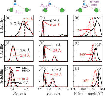
To this end, we take the HF clusters (dimer, tetramer, and pentamer) as the guiding example, because upon increasing the cluster size, the HB strength increases, and the influence of the NQEs switches from a tendency to lengthen to a tendency to shorten the intermolecular separations (as seen in Ref. [ 65 ]). The results are summarized in Fig.
 | Fig. 3. HF clusters as examples for detailed analysis of the QNEs. Distributions of the F–F distances (left), the F–H bond lengths (center), and the intermolecular bending (F–H···F angle, right) from MD (solid black lines) and PIMD (dashed red lines) for a selection of systems: the HF dimer (top), the HF tetramer (middle), and the HF pentamer (bottom). The MD and PIMD averages are shown in black and red vertical dashes, respectively. [ 7 ] |
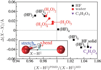
The above analysis provides a qualitative understanding of the trend observed. For a more rigorous examination of this picture and a quantitative description of this competition for all systems studied, we further calculate the projection ( X –H || ) of the donor molecule’s covalent bond along the intermolecular axis (see the inset of Fig.
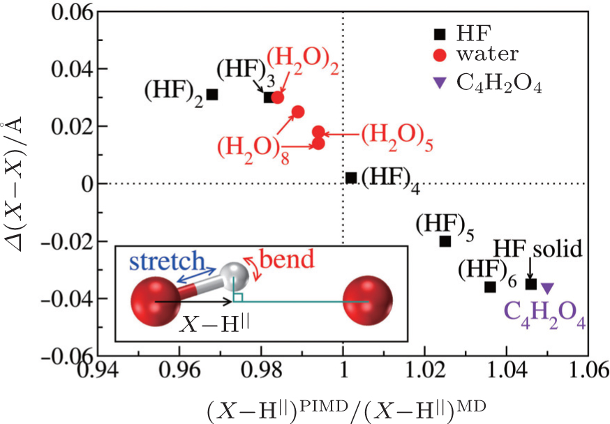 | Fig. 4. Quantification of the competition between the quantum fluctuations on the stretching and bending modes. The differences in average shortest heavy-atom distances between PIMD and MD simulations ( Δ ( X – X ), vertical axis) are plotted as a function of the ratio of the projection of the donor X –H covalent bond along the intermolecular axis from PIMD and MD simulations (horizontal axis). x larger (smaller) than 1 indicates a dominant contribution from the stretching (bending) mode when the NQEs are included. Negative values of Δ ( X – X ) indicate that NQEs decrease the intermolecular separation. An almost linear correlation between the two variables is observed. The inset illustrates the geometry used for projecting the donor covalent X –H bond onto the intermolecular axis. The curved red arrow represents the intermolecular bending and the straight blue arrow represents the intramolecular stretching. [ 7 ] |
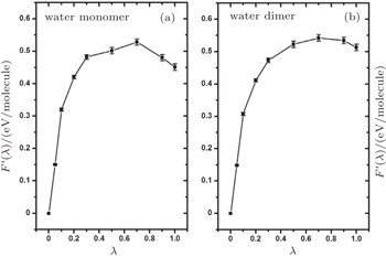
In Section 3, we have analyzed the influence of NQEs on the strength of HBs, taking the geometric changes as the indicator. A rigorous quantification of this influence, however, requires an explicit calculation of the contribution of the NQEs to the free energy of the H-bonded systems, using the method shown in Section 2. In Fig.

 | Fig. 5. Thermodynamic integration based on ab initio PIMD sampling for the calculation of the free-energy change due to NQEs in the water monomer and dimer. F ′( λ ) is as defined in Eq. ( |
HB is generally weak, but ubiquitous and essential to life on earth. The small mass of hydrogen means that many properties of HBs are quantum mechanical in nature, although quite often their theoretical descriptions remain classical. Due to the development of computer simulation methods, this influence of NQEs on the structural and energetic properties of some hydrogen bonded systems has been systematically studied in recent years. Here we present a review of these works, by focussing on the explanation of the main methods behind the simulations, i.e., the ab initio PIMD method as well as its extension in combination with the thermodynamic integration method for the calculation of the free energies. As a practical example of these studies, ab initio PIMD simulations on the structural properties of the hydrogen bonded systems have shown that the NQEs have a tendency to strengthen the strong HBs and weaken the weak ones, which could be explained by a competition of the quantum fluctuations on the stretching and bending modes.
| 1 | |
| 2 | |
| 3 | |
| 4 | |
| 5 | |
| 6 | |
| 7 | |
| 8 | |
| 9 | |
| 10 | |
| 11 | |
| 12 | |
| 13 | |
| 14 | |
| 15 | |
| 16 | |
| 17 | |
| 18 | |
| 19 | |
| 20 | |
| 21 | |
| 22 | |
| 23 | |
| 24 | |
| 25 | |
| 26 | |
| 27 | |
| 28 | |
| 29 | |
| 30 | |
| 31 | |
| 32 | |
| 33 | |
| 34 | |
| 35 | |
| 36 | |
| 37 | |
| 38 | |
| 39 | |
| 40 | |
| 41 | |
| 42 | |
| 43 | |
| 44 | |
| 45 | |
| 46 | |
| 47 | |
| 48 | |
| 49 | |
| 50 | |
| 51 | |
| 52 | |
| 53 | |
| 54 | |
| 55 | |
| 56 | |
| 57 | |
| 58 | |
| 59 | |
| 60 | |
| 61 | |
| 62 | |
| 63 | |
| 64 | |
| 65 |