Discovered in 1996 and named after the Spanish physicist Parrondo, Parrondo’s paradox states that setting up two losing games together can result in a winning scenario. ^{[ 1 , 2 ]} It means that, by alternating two losing strategies in a deterministic way, a positive game can be obtained. Symbolically, we thus have “losing + losing = winning”. For example, in a chess game, the sacrifice of some chess pieces can lead to winning a game; in the stock market, Parrondo’s game offers a possibility to make a profit by investing in losing stocks.

Though it looks contradictory and not every scientist agrees with its principle, ^{[ 3 ]} Parrondo’s paradox has still received a lot of attention and become an active topic in many research areas, such as minimal Brownian ratchet, ^{[ 4 ]} discrete-time ratchets, ^{[ 5 ]} game theory, ^{[ 6 ]} and molecular transport, ^{[ 7 ]} to name a few.

In receipt of the 1998 Steele Prize for Seminal Contributions to Research, Zeilberger responded that “... combining different and sometimes opposite approaches and viewpoints will lead to revolutions. So the moral is: Don’t look down on any activity as inferior, because two ugly parents can have beautiful children,...”. Indeed, we have witnessed a large number of research works showing the alternations of losing–winning, weakness–strength, order–chaos, and so on, in mathematical systems, control systems, quantum systems, biological systems, and physical systems. These counterintuitive results seem to be typical, not only in computational experiments but also in nature, where the underlying system dynamics are characterized by parameter switching either in an accidental or an intentional way. A review of Parrondo’s paradox can be found in Ref. [ 8 ] and the issues about Parrondo’s paradox were recently investigated in Ref. [ 9 ].

In Ref. [ 10 ], it was proven that Parrondo’s paradox can be generalized, for which a “winning” or “losing” result is obtained by combining N > 2 “losing” or (and) “winning” strategies. The generalization was modeled and demonstrated by applying a parameter switching (PS) algorithm onto nonlinear ordinary differential equations, ^{[ 10 – 12 ]} logistic map, ^{[ 13 ]} and fractals. ^{[ 14 ]}

In this paper, we adopt the PS algorithm to fractional-order differential equations (FDEs), aiming to extend the generalized Parrondo’s paradox to this interesting class of nonlinear systems. Recently, the fractional-order systems have received a lot of attention due to the fact that they are more accurate in modeling many practical systems (see Refs. [ 15 ]–[ 17 ]). Being a counterpart of the integer-order systems, the fractional-order systems are rich in complex dynamics, such as bifurcations, chaos, hyperchaos, etc. ^{[ 18 – 21 ]} The control and synchronization issues of these systems have also been studied. ^{[ 18 – 20 , 22 ]} To deal with the associated FDEs, different versions of fractional derivatives, such as Grunwald–Letnikov fractional derivative, Reimann–Liouville fractional derivative, and Caputo fractional derivative, ^{[ 23 ]} are possible. Since analytical solutions of nonlinear FDEs are usually not obtainable, the use of the numerical integration method such as the Adams–Basforth–Moulton predictor-corrector scheme (ABM) ^{[ 24 ]} is common. It is also possible to have a physical realization of the FDE which is mainly based on the frequency domain approximation. ^{[ 25 ]} This method has been widely applied, ^{[ 19 , 21 ]} yet there are still many arguments about the approximation. ^{[ 26 ]}

The rest of this paper is organized as follows. Section 2 describes the PS algorithm for FDEs. Section 3 presents the implementation of the PS algorithm for modeling the generalization of Parrondo’s game. The results are demonstrated with an example of fractional-order Chen’s system, in which Parrondo’s paradox generalization is considered. Finally, the conclusion section closes the paper.

Let us consider the following Caputo-type autonomous initial value problem (IVP)

Remark 1 (i) Recently, some researchers questioned the appropriateness of the use of the initial conditions in the Caputo derivative. These comments are more based on a philosophical point of view than a mathematical one (see Ref. [ 28 ]). On the other hand, it should be emphasized that, in practical (physical) problems, physically interpretable initial conditions are necessary. Thus, the Caputo derivative, as a fully justified tool, well suits this requirement, and the initial condition with fractional derivatives ^{[ 29 ]} can be avoided. (ii) The class of systems modeled by Eqs. ( 1 ) and (2) comprises systems of fractional-order Lorenz, Chen, Chua, Rössler, and many others.

In order to integrate numerically IVP ( 1 ), we adopt the fractional Adams–Bashforth–Moulton (ABM) method, which has been discussed in Ref. [ 29 ] and analyzed in detail in Ref. [ 30 ].

Given a set of parameters, with N ≥ 2, and weights m _i ∈ ℕ* associated with each p _i , the parameter p in Eq. ( 2 ) is switched within while the IVP is numerically integrated in the following manner: for the first m ₁ integration steps of length h (where h is the fixed step size specified in the fractional ABM), p = p ₁ ; for the next m ₂ steps, p = p ₂ ; and so on, until for the last m _N steps, p = p _N . The algorithm repeats with p = p ₁ for m ₁ steps, then with p = p ₂ for m ₂ steps, and so on, until the entire time interval I is covered.

Given N , , and weights m _i , i = 1,2, …, N , we hereafter simply denote the corresponding PS algorithm as

For example, the scheme [2 p ₁ , 1 p ₂ ] with a fixed h means that the IVP ( 1 ) is solved with p = p ₁ for the first two integration steps and p = p ₂ for the next step using numerical integration and so on.

By applying expression ( 3 ), the obtained “switched” solution of IVP ( 1 ) will converge to the solution of the “averaged” equation (referred to as the “averaged” solution) obtained for p = p * computed by

The convergence of the switched solution to the averaged solution under the PS algorithm for the integer-order systems can be proved with the average theorem ^{[ 10 ]} or based on the convergence of the used numerical method. ^{[ 11 ]} Numerically, the convergence can also be determined by characteristic tools for dynamical systems, such as checking the match between the two trajectories (switched and averaged) in phase plots, time series, Poincaré sections, etc, as for the fractional-order Chen system considered in this paper.

Remark 2 (i) As will be shown in Section 3, the value p * given by the relation ( 4 ) can be obtained in several ways, depending on and the weights m _i , i = 1,2,…, N , in scheme ( 3 ). (ii) By denoting , equation ( 4 ) can be rewritten as with . For any set and weights m _i , i = 1,2,…, N , p * is always within the interval ( p _min , p _max ) due to its convexity property, where and Reversely, the only condition to obtain a specific value of p * is to choose some set , such as p *∈ ( p _min , p _max ). (iii) The bounds for h are determined by the numerical integration method in-use (the fractional ABM utilized here).

The applications of the PS algorithm are wide. For example, it is possible to obtain the numerical approximation of some attractors of a system modeled by the IVP ( 1 ), whose parameter p = p̃ cannot be set for some reason. By choosing and m _i , i = 1,2,…, N , such that the right-hand side of Eq. ( 4 ) gives p̃ , the switched solution can lead to the targeted attractor corresponding to p̃ , with the use of the PS algorithm. It should also be noted that the simplicity of this approach, in providing an approximation of any solution of Eq. ( 1 ), resides in the linear dependence on p as given in the term p Ax .

Let us consider a system modeled by IVP ( 1 ) and assume that IVP ( 1 ) exhibits a characteristic behavior (attractor) which is either chaotic or regular for every , i = 1,2,…, N . Due to the uniqueness of solutions induced by the Lipschitz property, each p _i will correspond to a unique behavior denoted by chaos or order, given that the initial condition is fixed.

Now, the following notations for the numerically approximated attractors are defined (after neglecting first transients):

• A _{p i} denotes the attractor corresponding to p _i ;

• A * is the “switched attractor” obtained by the PS algorithm;

• A _{p *} is the “averaged attractor” obtained from IVP ( 1 ) with p = p *.

If in the known form of Parrondo’s paradox “losing + losing = winning”, we denote chaos := losing and order := winning, one obtains chaos + chaos = order. If one considers the system ( 1 ) for the case of N = 2 and , all possible cases obtained with the PS algorithm are tabulated in Table 1 . As observed, only the second and the fifth cases can be referred to as Parrondo’s paradox. In the second case, using the PS algorithm, the obtained attractor A * approximates the averaged attractor A _{p *} which is chaotic even though A _{p 1} and A _{p 2} are regular motions. In this case, one can affirm that the PS algorithm models the variant of Parrondo’s game: order ₁ + order ₂ = chaos. Reversely, in the fifth case, the resultant attractor by the PS algorithm, A *, approximates the averaged attractor A _{p *} , which is a regular motion, even if A _{p 1} and A _{p 2} are chaotic. This leads to another form of Parrondo’s game: chaos ₁ + chaos ₂ = order.

Table 1.

Table 1.

Table 1. Possible results with PS algorithm for N = 2. . A p 1 + A p 2 = A * Parranodo’s parradox order 1 + order 2 = order 3 No order 1 + order 2 = chaos Yes order 1 + chaos = order 2 No order + chaos 1 = chaos 2 No chaos 1 + chaos 2 = order Yes chaos 1 + chaos 2 = chaos 3 No

Table 1. Possible results with PS algorithm for N = 2. .

It is interesting to point out that specific attractor, either stable or chaotic, can be obtained with Parrondo’s paradox, despite the original behaviors corresponding to . By referring to the results in Table 1 , Parrondo’s paradox can be viewed as a kind of “chaos-control”-like or “anticontrol”-like action. The procedures are as follows: suppose that one intends to obtain a regular motion corresponding to some p *, which is unavailable starting from a set that generates only chaotic motions. Then, by choosing an adequate set of weights m _i such that the right-hand side of Eq. ( 4 ) gives the desired value p * (see Remark 2 (ii)), the desirable ordered motion can be approximated by the PS algorithm and one obtains a chaos-control-like phenomenon. If the desirable attractor is chaotic, and generates regular motions, Parrondo’s paradox is an analogy of the anticontrol-like phenomenon (see Ref. [ 32 ]). Obviously, relaxed forms of Parrondo’s paradox (cases 1, 3, 4, and 6 in Table 1 ) can be considered as control-like or anticontrol-like schemes.

When one considers a general case of N ≥ 2, the following property is held, stating the existence of the generalized Parrondo’s paradox.

Property 1 Consider a dynamical system modeled by the IVP ( 1 ), a set with N ≥ 2 and p * ∈ ( p _min , p _max ). Then, the following properties are obtained:

(i) If p * corresponds to a stable periodic motion, and is intercalated by some values of p _i belonging to some chaotic windows, then the following generalized Parrondo’s paradox exists:

(ii) If p * corresponds to a chaotic motion, and is intercalated by some values p _i belonging to some periodic windows, then the following generalized Parrondo’s paradox exists:

Proof The proof of (i) is given as follows. Assuming that elements in all belong to some different chaotic windows and p * ∈ ( p _min , p _max ), the convexity property of p * (Remark 2 (ii)) assures that, there exists a suitable set of weights, m _i , i = 1,2,…, N , such that equation ( 4 ) is satisfied. Under the convergence of the PS algorithm, the switched solution, determined by the values p _i , i = 1,2,…, N , will tend to the averaged solution corresponding to p = p *. As a result, the corresponding attractor A * will approximate the averaged attractor A _{p *} . That ends the proof of (i). The proof of (ii) can be obtained in a similar way.

Remark 3 As is known, the numerical methods for fractional-order equations consider the whole or partial history of the variables. Therefore, in the analytical proof of the convergence of the PS algorithm, which modifies these values at every integration step, this phenomenon has to be considered. On the other hand, the convergence for fractional-order systems can also be verified by characteristic computational tools for dynamical systems such as phase plots, time series, Poincaré sections, and so on.

In the following, we focus on the incommensurate fractional-order Chen system, ^{[ 32 ]} which can be expressed as

Fig. 1.

	Figure Option View Download New Window
	Fig. 1. Bifurcation diagram of fractional-order Chen’s system (5).

Fig. 2.

Figure Option View Download New Window

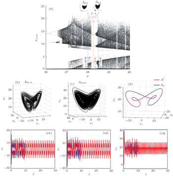
Fig. 2. Parrondo’s paradox (chaos-control-like): chaos 1 + chaos 2 = order, modeled by the PS algorithm under the scheme [1 p 1 , 1 p 2 ], with p 1 = 38.10 and p 2 = 38.50: (a) position of the underlying attractors in the parameter space, (b) phase plot of A p 1 , (c) phase plot of A p 2 , (d) phase overplot of the switched attractor A * (red) and the averaged attractor A p * (blue), (e) time series of A * and A p * .

We consider cases which model Parrondo’s variants, i.e., the chaos-control-like and chaos-anticontrol-like actions (the second and the fifth cases in Table 1 ) via the PS algorithm. The program code used to carry out the numerical integration of IVP ( 1 ) is an incommensurate variant of FDE12 in MATLAB, ^{[ 33 , 34 ]} implementing the fractional Adams–Bashfroth–Moulton method. The integration time interval is [0, 200], i.e., T = 200, and the step size is h = 0.002, which is commonly used in the fractional ABM method. ^{[ 30 ]}

In order to illustrate the match of the switched solution to the averaged solution, we overplot the underlying attractors in the phase space after ignoring the first transients. The matching between the two attractors shows the correctness of the results.

Let us first consider the stable cycle corresponding to p * = 38.30. The periodic cycle can be approximated with the PS algorithm, for example, using [ m ₁ p ₁ , m ₂ p ₂ ] with and m ₁ = m ₂ = 1 (Fig. 2(a) ). The corresponding chaotic attractors A _38.10 and A _38.50 are depicted in Figs. 2(b) and 2(c) , respectively. From Eq. ( 4 ), one can obtain p * = (1 × 38.10 + 1 × 38.50)/(1 + 1) = 38.30. As shown in Fig. 2(d) , by applying the PS algorithm, the switched attractor A * (plotted in red) well matches with the averaged attractor A _{p *} (in blue). The perfect match is also illustrated by overplotting the two time series, as given in Fig. 2(e) . Therefore, the existence of the following classical form of Parrondo’s paradox can be concluded:

Fig. 3.

	Figure Option View Download New Window
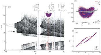
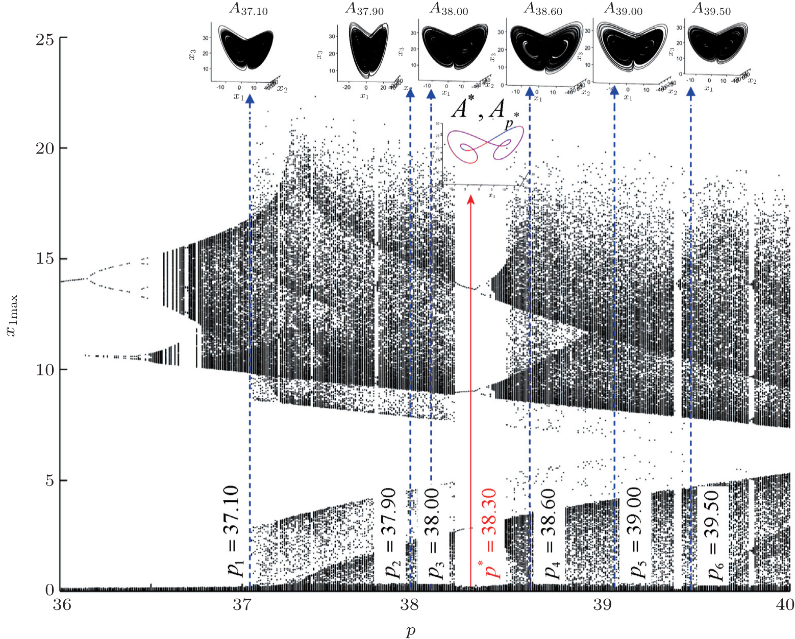
	Fig. 3. Generalized Parrondo’s paradox (chaos control-like): chaos 1 + … + chaos 6 = order, modeled by the PS algorithm under the scheme [2 p 1 ,3 p 2 ,1 p 3 ,2 p 4 ,3 p 5 ,1 p 6 ], with .

It should be emphasized that, the scheme for approximating an attractor is not unique, many different alternatives are possible with the PS algorithm (see Remark 2 (i)). For example, the same stable cycle in the previous example can be obtained by the scheme [2 p ₁ , 3 p ₂ , 1 p ₃ , 2 p ₄ , 3 p ₅ , 1 p ₆ ] with . It can be easily proved that the relation ( 4 ) leads to the same value of p * = 38.30. It is interesting to point out that the attractors, corresponding to elements in , are all chaotic while the obtained switching attractor is a stable cycle (Fig. 3 ). Thus, we have the following generalized Parrondo’s paradox:

The PS algorithm can be successfully numerically applied in many systems of fractional-order continuous or piecewise continuous (see the case of the new piecewise linear Chen system of fractional-order ^{[ 12 ]} ).

Fig. 4.

Figure Option View Download New Window

Fig. 4. Generalized Parrondo’s paradox (anticontrol-like): order 1 + order 2 + order 3 = chaos, modeled by the PS algorithm under the scheme [1 p 1 , 1 p 2 , 2 p 3 ], with : (a) position of the underlying attractors in the parameter space, (b) the switched attractor A * (red) and the averaged attractor A p * (blue) overplotted in the phase space, and (c) the Poincaré section of the attractors on the plane x 3 = 22.

We have shown via the PS algorithm that Parrondo’s paradox and its generalizations occur in fractional-order systems. By having N ≥ 2 bifurcation parameters, the PS algorithm leads to the generalized variant of Parrondo’s game: chaos ₁ + chaos ₂ + … + chaos _N = order, which can be considered as a chaos-control-like. Another form of generalized Parrondo’s paradox is order ₁ + order ₂ + … + order _N = chaos, which can be considered as a chaos-anticontrol-like. The simplicity of the PS algorithm resides in the linear dependence on p as given in the term p Ax . The Parrondo’s games are well illustrated numerically with the fractional-order Chen system. An open issue remains, i.e., to analytically prove the convergence of the PS algorithm for the case of fractional order nonlinear systems.