Quantum walks with coins undergoing different quantum noisy channels
Qin Hao 1 , Peng Xue 1, 2, †,
Department of Physics, Southeast University, Nanjing 211189, China
Beijing Institute of Mechanical and Electrical Space, Beijing 100094, China


† Corresponding author. E-mail: gnep.eux@gmail.com

Project supported by the National Natural Science Foundation of China (Grant Nos. 11174052 and 11474049) and the CAST Innovation Fund, China.

Abstract
Abstract

Quantum walks have significantly different properties compared to classical random walks, which have potential applications in quantum computation and quantum simulation. We study Hadamard quantum walks with coins undergoing different quantum noisy channels and deduce the analytical expressions of the first two moments of position in the long-time limit. Numerical simulations have been done, the results are compared with the analytical results, and they match extremely well. We show that the variance of the position distributions of the walks grows linearly with time when enough steps are taken and the linear coefficient is affected by the strength of the quantum noisy channels.

1. Introduction

The classical random walk (CRW) is well known due to its diverse applications in many fields, including designing algorithms in mathematics, describing diffusion processes in physics and biology, and stimulating the price fluctuation of stock market in finance. [ 1 3 ] Emerging as the quantum analogue of the CRW, the quantum walk (QW) has drawn intense investigation interest in recent years and exhibits striking nonclassical properties, among which the most important one is the ballistic spreading. Hereto, studies have shown that the QW has implications in various fields, such as quantum algorithm engineering, [ 4 8 ] quantum simulation, [ 9 17 ] universal quantum computing, [ 18 , 19 ] and energy transport in biology. [ 20 ] Experimentally, several different physical systems have been used to implement QWs, for instance, systems of trapped atoms or ions, [ 21 29 ] nuclear magnetic resonance, [ 30 , 31 ] and linear optics. [ 32 43 ] As real physical systems inevitably suffer from unwanted interactions with the environment, which show up as noise, research taking noise into account on QWs [ 44 , 45 ] is of practical value. QWs with noise have been extensively studied recently, mainly including the noise existing in the graphs on which the walker walks, [ 46 49 ] the noise caused by the interaction between the walker or the coin and the environment, [ 50 54 ] and the noise imposed on different coins used in the QWs. [ 55 58 ]

In this paper, we study discrete-time Hadamard QWs with coins undergoing different quantum noisy channels, including dephasing channel, bit flip channel, and depolarizing channel, which are of significance in quantum systems. By deducing the analytical expressions of the first two moments of position in the long-time limit and direct numerical simulations, we find that the variance of the position distribution of the walks grows linearly with time in the long-time limit, which means the QW is transmitted into the CRW. It indicates that noise which leads to decoherence plays a fundamental role in the transition from the quantum to the classical regime. Besides, the influence of the strength of quantum noise is found to be responsible for the linear coefficient.

This paper is organized as follows. In Section 2, we briefly review the perfect Hadamard QW. In Section 3, we present discrete-time QWs with coins undergoing three different types of quantum noisy channels (dephasing channel, bit flip channel, and depolarizing channel) respectively, and give the analytical expressions of the first two moments of position in the long-time limit. In Section 4, we analyze the results of numerical simulations compared with the analytical results. Finally, in Section 5, we summarize and give a conclusion.

2. Perfect Hadamard quantum walk

The perfect Hadamard QW is usually considered to be the simplest version of QW, which includes only one walker walking on a line and a two-dimensional quantum coin with no decoherence. Before each step is taken, the Hadamard operator is used for coin flipping. The walker takes a step left or right according to the coin state after the flipping, head or tail. The state of the walker is | x t ⟩, where x t is the coordinate of the walker’s position on the line after t steps. Starting from the origin of the line gives the initial state of the walker | x 0 ⟩ = |0⟩. The initial coin state is usually chosen to be The initial state of the system becomes | Φ 0 ⟩ = | x 0 ⟩ ⊗ | ϕ 0 ⟩. The step operator applied to the position state of the walker takes the form

where Ŝ , Ŝ are the conditional position shift operators on the walk’s position state

and 0 , 1 are projectors applied to the coin

The evolution operator of the system for one step of the walk then becomes

where Î w is the identity operator applied to the walker. Therefore, the final state of the system after t steps is

In order to obtain an analytical result, we perform a Fourier transformation from the position space to the momentum space

The state | k ⟩ is the eigenstate of Ŝ , Ŝ and satisfies the relations

The inverse Fourier transformation is given by

Thus, the initial state of the walker becomes

The evolution operator in the momentum space becomes

where Û k is a unitary operator applied to the coin state and takes the form

Meanwhile, the final state of the system in the momentum space can be expressed as

The solution to the QW of this case has been shown in Ref. [ 59 ] and the variance of the position distribution of the walk grows quadratically with time in the long-time limit, which is a general symbol for QWs.

3. Quantum walks with coins undergoing different noisy channels

Now we discuss the Hadamard QW with decoherence introduced via the coin undergoing quantum noisy channels on the basis of the reviewed content in the above section. The general form of quantum noise applied to the coin state is

where ρ c = | ϕ ⟩ ⟨ ϕ |, which is the density matrix of the initial coin state, is the density matrix of the coin state with noise involved, and the ensemble of  n represents the operation of noise, which satisfies

For the initial state of the system,

after one step, the state becomes

Similarly, after t steps, the state evolves to

Making use of the method in Ref. [ 58 ], we define a super-operator kk′ for the evolution of the QW system with noise, and kk′ satisfies

Moreover, kk′ possesses the property of trace preserving,

Then we rewrite Eq. ( 17 ) with kk′

The probability of the walker reaching position x after t steps is

The moment of the position distribution for the QW is

We use the relations below for further evaluating:

Besides, we have to use the formula

Due to the trace preserving property of kk′ , we redefine kk = k for simplicity. Thus, we have the following expressions for the first two moments of position:

In this paper, we consider three different quantum noisy channels. The general form of noise mapping on the coin state is

where is the Pauli matrix, , . Corresponding to , we have . The parameters for the dephasing channel take the form

The parameters for the bit flip channel take the form

The parameters for the depolarizing channel take the form

Here γ is the parameter related to the strength of the noisy channel and t is the time of the coin in the noisy channel. We choose γ and t both to be constant and define p = e γt , which means that the coin will be in the identical strength noisy channel for the same duration of time when each flipping is made. The new parameter p (0 ≤ p ≤ 1) also indicates the strength of the noisy channel involved. The larger the p , the smaller the strength of the noisy channel. From the definitions, it is obvious that if p = 1, there is no noise at all. An arbitrary two-by-two matrix can be written in the representation of the usual Pauli matrixes

For simplicity, the matrix can be represented as a column vector with being the base

Then k turns into

for the dephasing channel, bit flip channel, and depolarizing channel, respectively. With the representation of the Pauli matrixes, the processes of left multiplying and right multiplying by are given by matrixes Z L and Z R ,

Then we go back to Eq. ( 29 ) for the first moment of position

We use the form of the column vector from Eq. ( 33 ) to represent the initial coin state and the values for r 0 , r 1 , r 2 , r 3 are decided by the initial coin state chosen. In the long-time limit, because the eigenvalues of k satisfy 0 < | λ | < 1. Thus, the first moment approximately turns to

Similarly, we apply Eqs. ( 37 ) and ( 38 ) to Eq. ( 30 ) for the second moment

where approaches zero in the long-time limit. For different quantum noisy channels, we obtain different forms of k and respectively substitute k 1 , k 2 , k 3 for k in Eqs. ( 40 ) and ( 41 ). For the dephasing channel, we obtain

Furthermore, the variance of the position distribution of the QW is given by

For the bit flip channel, we obtain

The variance for the bit flip channel turns out to be

For the depolarizing channel, we obtain

Then the variance for the depolarizing channel is

Although the first two moments of position have different forms for different quantum noisy channels, we find some properties in common from the results above. The first moment is dependent on the initial state while the second moment is not. The variance grows linearly with time in the long-time limit for all three quantum noisy channels, which indicates that the QW has transmitted to the CRW. However, the rate of growth is different, which also depends on the strength of the noisy channel and will be discussed in the next section.

4. Numerical simulations and analysis

We simulate the QWs according to the expression

where n = Πw  n denotes the operator of noise in the system. Further, we calculate the variance of the position distribution of the QW with coins undergoing different noisy channels. We also choose four different noisy strengths, p 2 = 0.2, 0.4, 0.6, 0.8, for each noisy channel. For simplicity and fair comparison among different noisy channels, we choose the initial state of the coin to be for all cases. The results of numerical simulations are shown in Figs. 1 3 for the dephasing channel, bit-flip channel, and depolarizing channel, respectively.

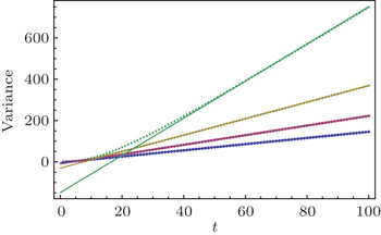
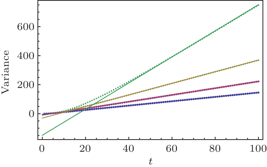
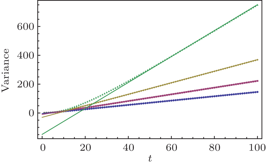
Fig. 1. Variance versus t for the Hadamard QWs with coins undergoing dephasing channel. The strengths of the noisy channel are p 2 = 0.2 (blue), 0.4 (purple), 0.6 (yellow), and 0.8 (green). Solid lines are results from the analytical solutions while the points are from numerical simulations. For all cases, the initial state of the coin is .
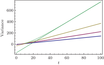
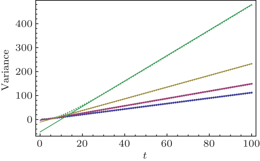
Fig. 2. Variance versus t for the Hadamard QWs with coins undergoing the bit-flip channel. The strengths of the noisy channel are p 2 = 0.2 (blue), 0.4 (purple), 0.6 (yellow), and 0.8 (green). Solid lines are results from the analytical solutions while the points are from numerical simulations. For all cases, the initial state of the coin is .

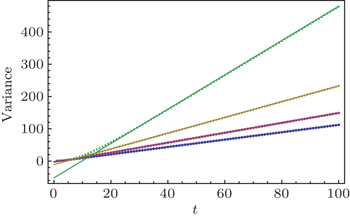
We can clearly see that the variance of the position distribution of the QW grows linearly with time when enough steps are taken. However, we can still see a quadratic growth of the variance in the first several steps, which is significantly different from that in the CRW and is usually considered as a qualitative mark for the quantumness of the QW system. On one hand, the quantumness of the walks stays for longer time with larger p 2 , which means the weakening of the strength of different noisy channels. On the other hand, for the same p 2 , the walk undergoing depolarizing channel takes less steps in the transition from the quantum to the classical regime than that undergoing dephasing channel and bit-flip channel, the results of which are identical for the initial state we choose. Although the steps for the quantum-to-classical transition of the walks are dependent on both the value of p 2 and the type of noisy channel, the number of steps is 100 in our simulations and is obviously big enough for all cases we choose to see the linear growth of variance with time of the walks, which is also confirmed by the fact that the analytical expressions we find in the long time limit match extremely well with the results of numerical simulations. Besides, the linear growth coefficient of variance versus t increases gradually with p 2 , and the linear growth coefficient of variance for the dephasing channel and bit-flip channel is larger than that for the depolarizing channel with the same noisy strength.

Fig. 3. Variance versus t for the Hadamard QWs with coins undergoing depolarizing channel. The strengths of the noisy channel are p 2 = 0.2 (blue), 0.4 (purple), 0.6 (yellow), and 0.8(green). Solid lines are results from the analytical solutions while the points are from numerical simulations. For all cases, the initial state of the coin is .
5. Conclusion

We have studied the Hadamard QWs with coins undergoing different quantum noisy channels, including dephasing channel, bit-flip channel, and depolarizing channel. We find the analytical expressions of the first two moments of position in the long-time limit, which match extremely well with the results of the numerical simulations. We show that the variance of the position distribution of the QW grows linearly with time when enough steps are taken, and still exhibits a quadratic growth in the first several steps, which is an important sign of QWs. The linear growth coefficient of variance versus the steps of the walks increases gradually with the weakening of the noise in different noisy channels. It is decoherence transmitting the QW to the classical.

Reference
1 Barber M 1970 Random and Restricted Walks: Theory and Applications New York Gordon and Breach
2 Berg H C 1993 Random Walks in Biology Princeton Princeton Univ. Press
3 Fama E F 1995 Financ. Anal. J. 51 75
4 Dür W Raussendorf R Kendon V M Briegel H 2002 Phys. Rev. A 66 052319
5 Ambainis A 2003 Int. J. Quantum Inf. 1 507
6 Childs A M Cleve R Deotto E Farhi E Gutmann S Spielman D A 2003 Proc. 35th ACM Symposium on Theory of Computing 59 68
7 Shenvi N Kempe J Whaley K B 2003 Phys. Rev. A 67 052307
8 Kempe J 2003 Contempo. Phys. 44 307
9 Zhang R Xu Y Xue P 2015 Chin. Phys. B 24 010303
10 Zhang R Xue P 2014 Quant. Inf. Process. 13 1825
11 Xue P Sanders B C 2013 Phys. Rev. A 87 022334
12 Xue P Sanders B C 2012 Phys. Rev. A 85 022307
13 Brun T A Carteret H A Ambainis A 2003 Phys. Rev. Lett. 91 130602
14 Kitagawa T Rudner M S Berg E Demler E 2010 Phys. Rev. A 82 033429
15 Xue P Sanders B C 2013 Phys. Rev. A 87 022334
16 Zhang R Xue P Twamley J 2014 Phys. Rev. A 89 042317
17 Zhan X Qin H Bian Z H Li J Xue P 2014 Phys. Rev. A 90 012331
18 Childs A M 2009 Phys. Rev. Lett. 102 180501
19 Childs A M Gosset D Webb Z 2013 Science 339 791
20 Sension R J 2007 Nature 446 740
21 Xue P Sanders B C Leibfreid D 2009 Phys. Rev. Lett. 103 183602
22 Xue P Sanders B C 2008 New J. Phys. 10 053025
23 Xue P Sanders B C Blais A Lalumiere K 2008 Phys. Rev. A 78 042334
24 Xue P 2013 The Journal of Computational and Theoretical Nanoscience: Special Issue: Theoretical and Mathematical Aspects of the Discrete Time Quantum Walk 10 1
25 Qin H Xue P 2014 Chin. Phys. B 23 010301
26 Genske M Alt W Steffen A Werner A H Werner R F Meschede D Alberti A 2013 Phys. Rev. Lett. 110 190601
27 Zahringer F Kirchmair G Gerritsma R Solano E Blatt R Roos C F 2010 Phys. Rev. Lett. 104 100503
28 Schmitz H Matjeschk R Schneider C Glueckert J Enderlein H Huber T Schaetz T 2009 Phys. Rev. Lett. 103 090504
29 Karski M Forster L Choi J M Steffen A Alt W Meschede D Widera A 2009 Science 325 174
30 Du J Li H Xu X Shi M Wu J Zhou X Han R 2003 Phys. Rev. A 67 042316
31 Ryan C A Laforest M Boileau J C Laflamme R 2005 Phys. Rev. A 72 062317
32 Xue P Zhang R Qin H Zhan X Bian Z Li J Sanders B C 2015 Phys. Rev. Lett. 114 140502
33 Bian Z Li J Qin H Zhan X Zhang R Sanders B C Xue P 2015 Phys. Rev. Lett. 114 203602
34 Peruzzo A Lobino M Matthews J C F Matsuda N Politi A Poulios K Zhou X Lahini Y Ismail N Worhoff K Bromberg Y Silberberg Y Thompson M G Obrien J L 2010 Science 329 1500
35 Schreiber A Gabris A Rohde P P Laiho K Stefanak M Potocek V Hamilton C Jex I Silberhorn C 2012 Science 336 55
36 Broome M A Fedrizzi A Lanyon B P Kassal I Aspuru-Guzik A White A G 2010 Phys. Rev. Lett. 104 153602
37 Schreiber A Cassemiro K N Potocek V Gabris A Mosley P J Andersson E Jex I Silberhorn C 2010 Phys. Rev. Lett. 104 050502
38 Sansoni L Sciarrino F Vallone G Mataloni P Crespi A Ramponi R Osellame R 2012 Phys. Rev. Lett. 108 010502
39 Solntsev A S Sukhorukov A A Neshev D N Kivshar Y S 2012 Phys. Rev. Lett. 108 023601
40 Kitagawa T Broome M A Fedrizzi A Rudner M S Berg E Kassal I Aspuru-Guzik A Demler E White A G 2012 Nat. Commun. 3 882
41 Crespi A Osellame R Ramponi R Giovannetti V Fazio R Sansoni L Nicola F D Sciarrino F Mataloni P 2013 Nat. Photon. 7 322
42 Xue P Qin H Tang B 2014 Sci. Rep. 4 4825
43 Xue P Qin H Tang B Sanders B C 2014 New J. Phys. 16 053009
44 Xue P Zhang Y S 2013 Chin. Phys. B 22 070302
45 Zhang R Qin H Tang B Xue P 2013 Chin. Phys. B 22 110312
46 Zhao J Tong P 2015 Quant. Inf. Process. 14 2357
47 Santos R A M Portugal R Fragoso M D 2014 Quant. Inf. Process. 13 559
48 Oliveira A C Portugal R Donangelo R 2006 Phys. Rev. A 74 012312
49 Sanders B C Bartlett S D Tregenna B Knight P L 2003 Phys. Rev. A 67 042305
50 Xu Y Y Zhou F Chen L Xie Y Xue P Feng M 2012 Chin. Phys. B 21 040304
51 Schreiber A Cassemiro K N Potocek V Gabris A Jex I Silberhorn C 2011 Phys. Rev. Lett. 106 180403
52 Liu C Petulante N 2011 Phys. Rev. A 84 012317
53 Annabestani M Akhtarshenas S J Abolhassani M R 2010 Phys. Rev. A 81 032321
54 Yin Y Katsanos D E Evangelou S N 2008 Phys. Rev. A 77 022302
55 Xiong S Yang W S 2013 J. Stat. Phys. 152 473
56 Banerjee S Srikanth R Chandrashekar C M Rungta P 2008 Phys. Rev. A 78 052316
57 Kosik J Buzek V Hillery M 2006 Phys. Rev. A 74 022310
58 Brun T A Carteret H A Ambainis A 2003 Phys. Rev. A 67 032304
59 Nayak A Vishwanath A 2000 e-print quant-ph/0010117