The ideal charged Bose gas (CBG) consists of a gas of spin-less, charged bosons coupled to an external homogeneous magnetic field has played a significant role in understanding lots of exotic quantum phenomena including superfluidity and superconductivity. The study of the CBG has a long history and it is impossible to give a complete list here. Perhaps, the first investigation in three dimensions was performed more than half a century ago by Osboren, ^{[ 1 ]} and then by Schafroth ^{[ 2 ]} who showed that Bose–Einstein condensation (BEC) ^{[ 3 – 7 ]} cannot exist at any finite temperature in the presence of a homogeneous magnetic field. However, the system does exhibit the essential equilibrium features of a superconductor such as the Meissner–Ochsenfeld (MO) effect at lower temperatures in a magnetic field. May ^{[ 8 , 9 ]} extended this idea to a D -dimensional CBG and pointed out the BEC in CBG can take place only if D ≥ 5. Toms ^{[ 10 , 11 ]} subsequently argued that BEC cannot occur in the CGB in any spatial dimension D , while Rojas ^{[ 12 ]} has pointed out that BEC can take place with a diffuse transition. May’s work was confirmed and extended by Daicic and Frankel. ^{[ 13 ]} A semiclassical approach was used by Bayindir and Tanatar ^{[ 14 ]} to conclude that BEC can occur in the CBG in a magnetic field and in the presence of a crossed electric field. The thermodynamic properties of the 2D CBG in a magnetic field has also been investigated by van Zyl and Hutchinson. ^{[ 15 ]}

In recent years, with rapid progress in ultracold atoms, there has been a renewed interest in charged bosons. In a properly designed laser field, the center-of-mass (CM) motion of neutral atoms may mimic the dynamics of a charged particle in a magnetic field. ^{[ 16 ]} Alternatively, one can spin up the neutral atoms by confining them in a rotating frame. ^{[ 17 ]} Since the atomic gases of the experiments for BEC are dilute, as a first approximation the ideal Bose gas is a good starting model to explore theoretically in terms of basic interatomic interactions. Although not the focus of rotating Bose gases research, the thermodynamic properties of the rotating ideal Bose gases have also been studied by various authors. ^{[ 18 – 23 ]} In particular, the ideal CGB in a magnetic field was taken as an example to investigate the thermodynamic properties of rotating ideal Bose gases by the authors of Ref. [ 24 ]. The system they considered is placed in a uniform magnetic field and a harmonic trap

However, it is well known that in real experiment conditions, the number of trapped atoms N is finite ranging from a few thousand ^{[ 25 ]} to a few million, ^{[ 26 ]} the thermodynamic limit approximation may not be available. Actually, there are quite a lot of works dealing with this issue for the Bose gases. ^{[ 27 – 35 ]} Hence, in this paper we investigate the effects of a finite number of particles on the thermodynamic properties of an ideal charged Bose gas confined in an anisotropic harmonic potential and a constant magnetic field. Using an accurate density of states, we first calculate analytically the thermodynamic potential, then various thermodynamic properties including the Bose–Einstein transition temperature, the specific heat, and magnetization are analyzed. The corrections to these quantities due to the effects of a finite number of particles are also given explicitly. In particular, we show that the BEC condensation temperature is relevant to the magnetic field and the magnetization varies with the temperature when the particle number is finite. These behaviors are quite different from the infinite particle number case.

The rest of the paper is organized as follows. In Section 2, we introduce the Hamiltonian of the system and give the energy spectrum. The thermodynamic potential and various thermodynamic potentials are obtained and analyzed in Section 3, concluding remarks are made in the last section.

The ideal charged Bose gas we consider consists of N bosons with mass m and charge e > 0, is trapped in a harmonic confining potential which is anisotropic in all three dimensions ^{[ 26 , 36 ]} described by

The corresponding eigenfunctions for the Hamiltonian of Eq. ( 5 ) are also known, we refer the reader to Ref. [ 37 ] for more details. The behaviors of the frequencies ω _2,1 as functions of the strength of magnetic field B are plotted in Fig. 1 . In the case of isotropic harmonic potential, i.e., ω _x = ω _y = ω ₀ , then ω _1,2 = ω ∓ ω _c /2 with . In Fig. 2 , we plot the in-plane energy levels E _{n 1 n 2} as a function of the cyclotron frequency ω _c = eB /( mc ).

Fig. 1.

	Figure Option View Download New Window
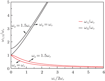
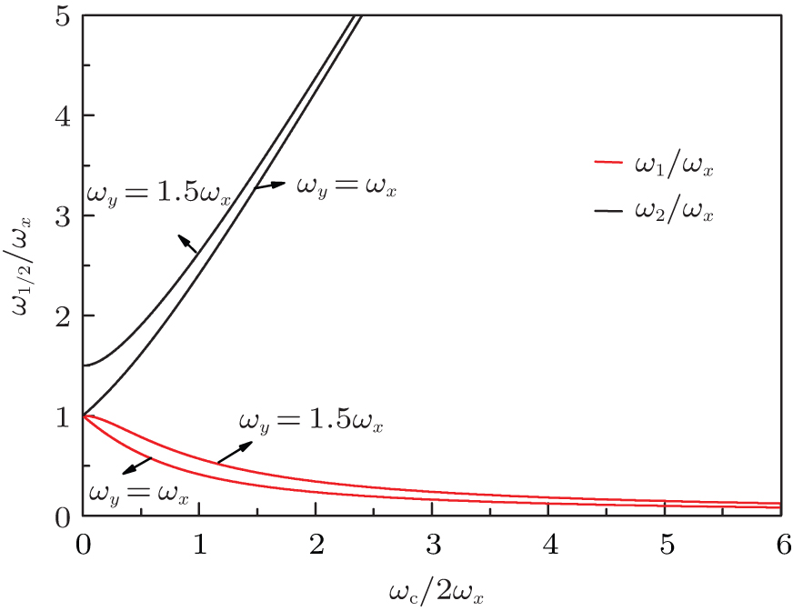	Fig. 1. The ω 1,2 / ω x as functions of the cyclotron frequency ω c = eB /( mc ) (in units of 2 ω x ), which is proportional to the strength of the magnetic field B .

Fig. 2.

	Figure Option View Download New Window
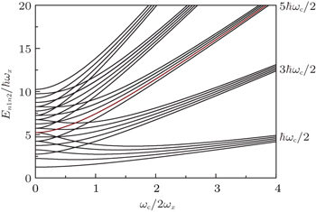
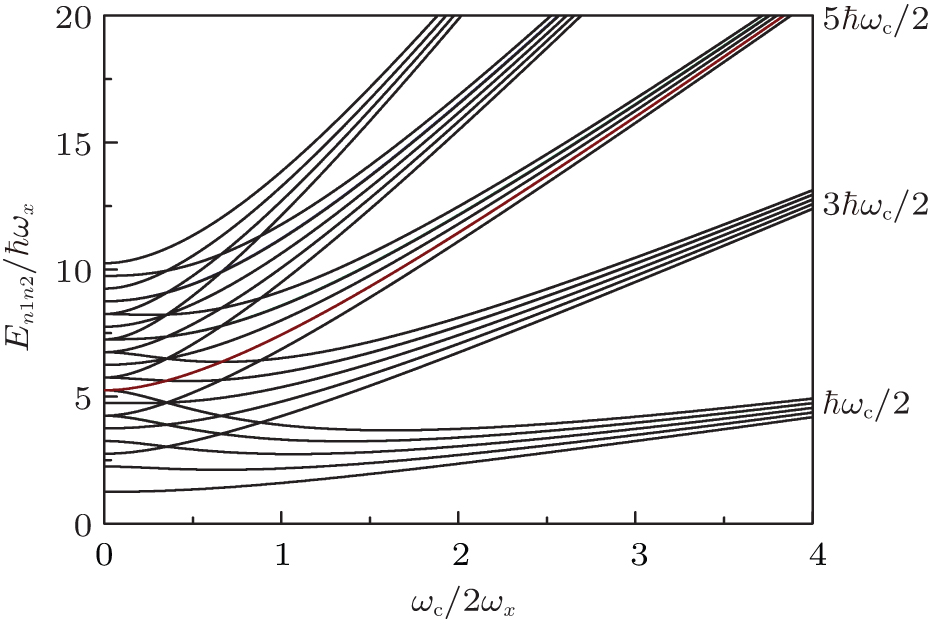	Fig. 2. The in-plane energy levels E n 1 n 2 (in units of ħω x ) as functions of the cyclotron frequency ω c = eB /( mc ) (in units of 2 ω x ), which is proportional to the strength of the magnetic field B .

Hence, the energy levels of the total model Hamiltonian are

In this section, we first calculate the thermodynamic potential, then the transition temperature and condensate fraction are obtained by taking into account the fact that the particle number N is finite. Finally, we calculate the specific heat and magnetization.

3.1. Thermodynamic potential

The thermodynamic potential of the system is ^{[ 38 ]}

where β = ( k _B T ) ⁻¹ is the inverse temperature, z = e ^{β ( μ − E ₀ )} . The above expression usually can be written as two parts

where the first part Ω ₀ = ln(1 − z )/ β , which is present only when there is a nonzero condensate. Alternatively, this part can also be described by using a background field Ψ ( r ), ^{[ 39 , 40 ]}

Notice here is the gauge-covariant derivative. The nonzero value of the background field Ψ which signals a condensate satisfies the following equation:

Thus we can expand Ψ ( r ) as Ψ ( r ) = ∑ _n C _n Ψ _n ( r ), where Ψ _n ( r ) are stationary state solutions to the Schrödinger equation

and they form a complete set. Since equation ( 13 ) is exactly the Schrödinger equation for the Hamiltonian of Eq. ( 4 ), one immediately realizes that E _n coincides with the single particle energy E _{n 1 n 2 n 3} of Eq. ( 8 ) with n = { n ₁ n ₂ n ₃ }. The corresponding eigenfunctions are also readily identified as

The coefficients C _n are determined by

When the temperature is above the BEC temperature T _c , the chemical potential μ is less than the ground state energy, μ < E ₀ . Thus, E _n ‒ μ ≠ 0 and C _n = 0 for all levels. As the temperature decreases, the chemical potential μ increases and reaches E ₀ at or below T _c . Then C ₀ ≠ 0 becomes the only nonzero solution of all C _n , which means the corresponding condensate wave function is Ψ ( r ) = C ₀ Ψ ₀ ( r ), with

where Φ ₀₀ ( x , y ) is the ground state wave function for H _xy , ^{[ 37 ]}

with

and

The second part of the thermodynamic potential is

where denotes the summation over all the eigenstates except the ground state. After expanding the logarithm, equation ( 22 ) can be expressed as a sum over the Bose–Einstein distribution function as

where g ( ϵ ) = ∑ _{n 1 n 2 n 3} δ( ϵ − ϵ _{n 1 n 2 n 3} ) is the density of the states (DOS). In the following we adopt an approximate but very accurate expression for the DOS as in Refs. [ 27 ] and [ 29 ]

where , and with . Note that γ is a function of B even in the isotropic case. Inserting Eq. ( 24 ) into Eq. ( 23 ) yields

where is the usual Bose–Einstein function. ^{[ 36 ]}

3.2. Transition temperature and condensate fraction

Having obtained the analytical expression for the thermodynamic potential in the above subsection, we next proceed to calculate the expression for the particle number N which can be derived via the equation N = − ∂Ω / ∂μ . The transition temperature and condensate fraction then can be obtained from the equation for the particle number.

Employing Eqs. ( 10 ) and ( 25 ), we can express the particle number as the summation of two parts

where

is the number of particles condensed on the ground state which is nonzero only when the temperature is lower than the transition temperature T ≤ T _c , and

is the particle number in the excited states.

When T = T _c , the number of particles condensed on the ground state is pretty large N ₀ ≫ 1 but still N ₀ ≪ N . Hence we can ignore N ₀ in Eq. ( 26 ) and from Eq. ( 27 ) we have z = N ₀ /( N ₀ + 1) ≈ 1, consequently we have

where ζ ( n ) = g _n (1) is the Riemann zeta function. The above equation can be readily solved and we obtain the transition temperature as

Note here, in the thermodynamic limit, the second term in the bracket of Eq. ( 30 ) can be dropped and the transition temperature becomes

which is irrelevant to the strength of the magnetic field. It should be pointed out that the transition temperature obtained in Ref. [ 24 ] is just Eq. ( 31 ). Hence, clearly they have taken the thermodynamic limit N → ∞.

Combining Eqs. ( 30 ) and ( 31 ), we have

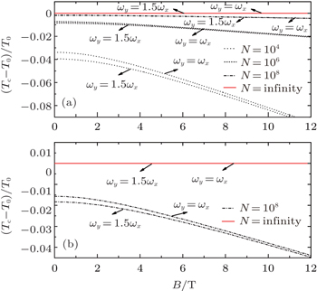
We plot the ratio ( T _c − T ₀ )/ T ₀ as a function of the strength of the magnetic field B in Fig. 3 . It is clear from the graph that the ratio decreases as B increases. Meanwhile, as the degree of anisotropic ω _y / ω _x increases at fixed ω _x the ratio also decreases.

Fig. 3.

	Figure Option View Download New Window
	Fig. 3. (a) The ( T c − T 0 )/ T 0 as a function of the strength of the magnetic field B for ω x = ω y and ω y = 1.5 ω x . We set N = 10 4 ,10 6 , 10 8 , ∞ and ω x = ω z = 10 3 Hz in the plots. In order to see the N = 10 8 curve in panel (a) clearly, we replot it in panel (b) with a different vertical scale.

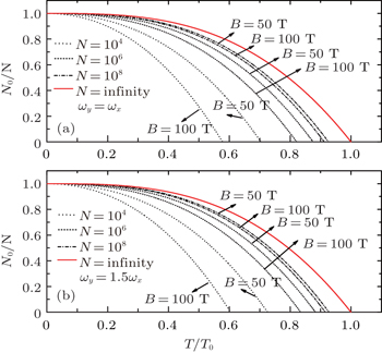
Next, let us examine the condensate fraction, i.e., the ratio of the number of condensate particles to the total particle number for T < T _c . Since N ₀ ≫ 1 in this case, we may substitute z ≈ 1 in Eq. ( 26 ) to obtain

or using the expression for T ₀ of Eq. ( 31 ), the above equation can be rewritten as

A plot of N ₀ / N as a function of ( T / T ₀ ) for different fixed values of the strength of the magnetic field B and particle number N is given in Fig. 4 . It is interesting to note that, in the case when N → ∞, equation ( 34 ) reduces to

thus the change of the B will not affect N ₀ / N . While in the finite particle number case, it is evident that when the value of B increases or N decreases, the value of N ₀ / N will be lowered as shown in Fig. 4 . In order to make the curves distinguishable, we set B = 50 T, 100 T in the graphs.

Fig. 4.

	Figure Option View Download New Window
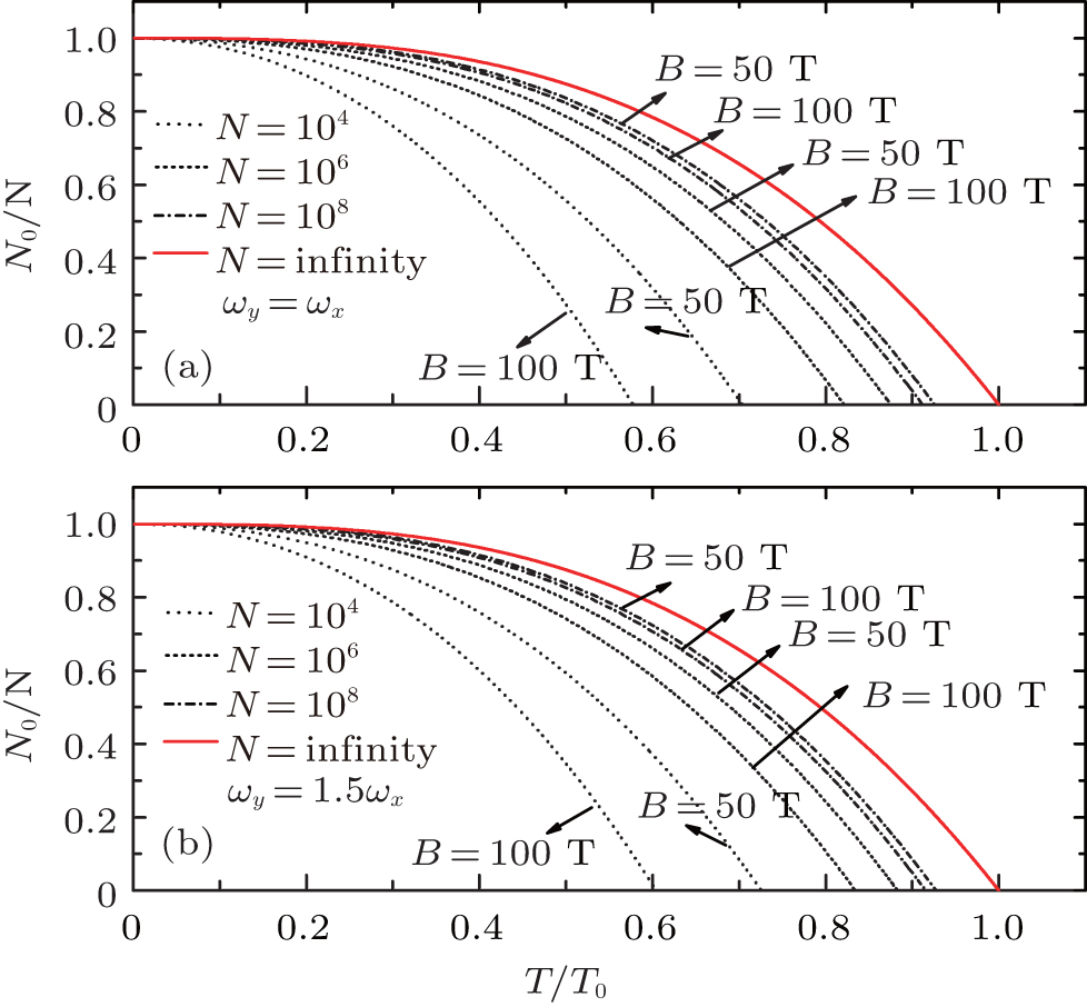	Fig. 4. The N / N 0 as a function of T / T 0 for different values of B = 50 T, 100 T or ω c = 29.606 kHz, 59.212 kHz, and N = 10 4 , 10 6 , 10 8 ,∞, ω x = ω z = 10 3 Hz. In panel (a) we set ω y = ω x , and ω y = 1.5 ω x in panel (b).

3.3. Chemical potential

In this subsection, we investigate the chemical potential μ , or equivalently z = e ^{β ( μ − E ₀ )} . Since it is clear when T ≤ T _c , μ = E ₀ , we only need to find out μ when T > T _c . As discussed earlier, N ₀ = 0 when T > T _c , hence, equation ( 26 ) can be rewritten as

which cannot be solved analytically. In order to obtain z as a function of ( N,B,T ), we solved Eq. ( 35 ) numerically and plot z and μ as functions of the temperature T/T ₀ for different values of the B and N in Figs. 5 and 6 . From the graphs, it is clear that in the region T > T _c , z and μ die down very fast as T increases. As shown in Fig. 6 , μ dies down faster as the particle number increases.

Fig. 5.

	Figure Option View Download New Window
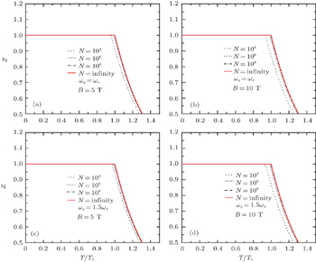
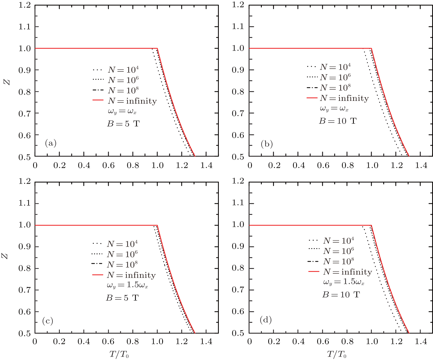	Fig. 5. The z as a function of T / T 0 for different values of B = 5 T, 10 T or ω c = 2.9606 kHz, 5.9212 kHz, N = 10 4 , 10 6 , 10 8 , ∞, and ω x = ω z = 10 3 Hz. We set ω y = ω x in panels (a) and (b) and ω y = 1.5 ω x in panels (c) and (d).

Fig. 6.

	Figure Option View Download New Window
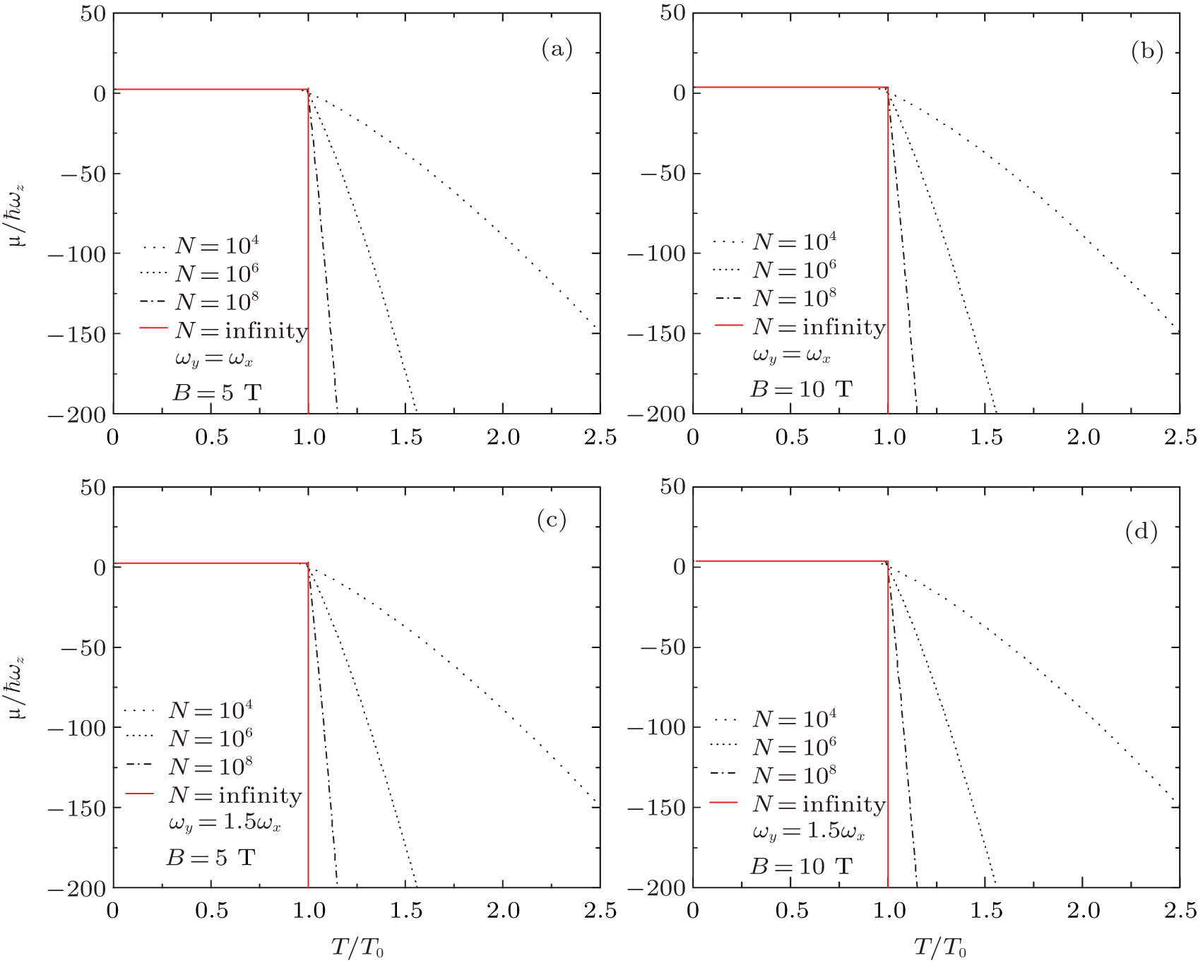	Fig. 6. Chemical potential μ as a function of T / T 0 for different values of B = 5 T, 10 T and N = 10 4 , 10 6 , 10 8 ,∞, ω x = ω z = 10 3 Hz. We set ω y = ω x in panels (a) and (b) and ω y = 1.5 ω x in panels (c) and (d).

In the thermodynamic limit N ≫ 1, we can ignore the last term of Eq. ( 35 ). Therefore, when T > T _c we have

where is the inverse function of g ₃ ( z ). From Eq. ( 36 ), it is easy to obtain that

From Fig. 5 , we note that in the regime T > T _c , only when N ₀ = 0, z = N ₀ /( N ₀ +1) ≪ 1 and g ₃ ( z ) ≈ z = e ^{β ( μ − E ₀ )} , equation ( 37 ) reduces to μ ≈ E ₀ − 3 k _B T ln( T/T ₀ ). However, there exists a transition region where the approximation z ≪ 1 is not valid, then we have to use Eq. ( 37 ) to obtain the value of μ .

3.4. Specific heat

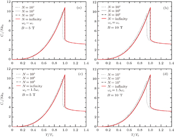
In this subsection we calculate the specific heat. The specific heat can be calculated by differentiating the internal energy U with respect to the temperature C _v ( T ) = ∂U / ∂T . The internal energy is given by

When T ≤ T _c , then z ≈ 1 and the above equation reduces to

thus the specific heat blow T _c is

When T > T _c , the specific heat can be obtained from Eq. ( 38 ) directly,

We plot the specific heat as a function of T / T ₀ for different values of B and N in Fig. 7 . It is clear from the graphs that when N is finite, the specific heat exhibits a continuous change. While in the limit of N → ∞, T _c = T ₀ , the specific heat shows an almost discontinuous jump at the transition temperature. When the particle number decreases, the maximum value of the specific heat decreases, and the whole curve moves left as the value of T _c decreases.

Fig. 7.

	Figure Option View Download New Window
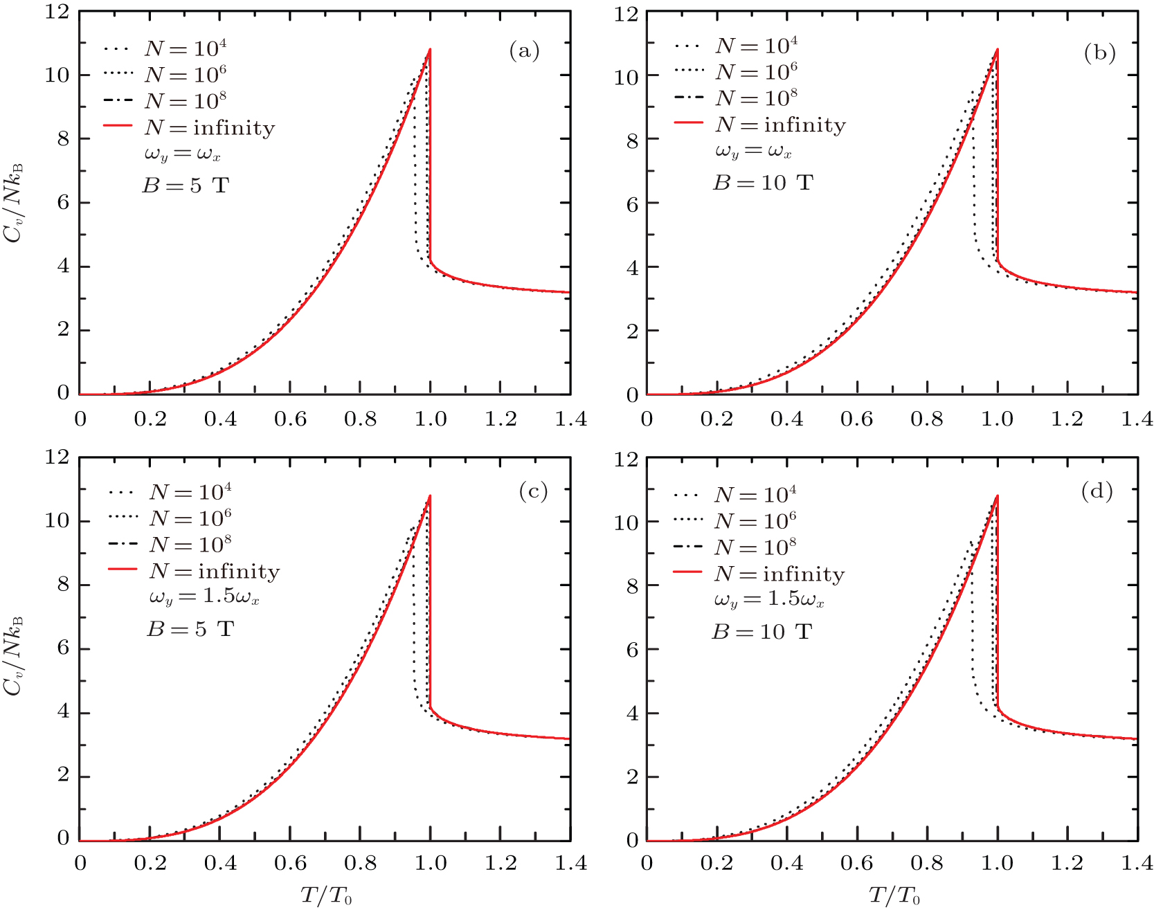	Fig. 7. The C v /( Nk B ) as a function of T / T 0 for different values of B = 5 T, 10 T, N = 10 4 , 10 6 , 10 8 , ∞, and ω x = ω z = 10 3 Hz. We set ω y = ω x in panels (a) and (b) and ω y = 1.5 ω x in panels (c) and (d).

3.5. Magnetization

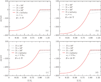
Similarly, the magnetization can be obtained from the thermodynamic potential

Hence, when T < T _c , it has two parts

where

Since z ≈ 1 when T < T _c , equation ( 42 ) becomes

or equivalently,

The magnetization for T > T _c can also be obtained readily

or

The magnetization M as functions of T / T ₀ for different values of B and N is plotted in Fig. 8 . As clearly reflected in the graphs, the magnetization M varies with the temperature and the diamagnetism is stronger at lower temperatures. This result is different from those obtained in Ref. [ 24 ], their magnetization stays invariant at all temperatures. Actually, if one takes the thermodynamic limit N → ∞, then the second terms in Eqs. ( 44 ) and ( 46 ) can be dropped and we would obtain the result that magnetization remains invariant at all temperatures.

Fig. 8.

	Figure Option View Download New Window
	Fig. 8. Magnetization M as a function of T / T 0 for different values of B = 5 T, 10 T, and N = 10 4 , 10 6 , 10 8 , ∞, ω x = ω z = 10 3 Hz. We set ω y = ω x in panels (a) and (b) and ω y = 1.5 ω x in panels (c) and (d).

From the expressions above, we can see that the magnetization M does depend on B , since ∂γ / ∂B ≠ 0. This point is clearly reflected in Fig. 8 . Moreover, magnetization above T _c is different from that below T _c , this is different from the results in Ref. [ 24 ]. Actually this difference originated from Eq. ( 30 ), where we have kept the N ^2/3 term, i.e. this is due to the finiteness of the particle number.

First, M/N as a function of T/T ₀ (Eqs. ( 44 ) and ( 47 )) appears to be the same for any value of particle number N . However, since the transition temperature depends on N , they are different for different values of N . It is worth stressing that M/N is a smooth function at T _c when N → ∞, this is quite different from the specific heat curve. On the other hand, from Eqs. ( 45 ) and ( 47 ), we know that M vanishes as B reduces to zero at all temperatures implying that Meissner–Ochsenfeld effect does not exist in an anisotropic harmonically trapped CBG. This result agrees with those obtained in Ref. [ 24 ].

In summary, by employing an accurate density of states, we calculate analytically the thermodynamic potential of an ideal charged Bose gas confined in an anisotropic harmonic potential and a constant magnetic field. Then we obtained the expressions for the Bose–Einstein transition temperature, condensate fraction, the specific heat and magnetization taking into account the fact that the particle number N is finite. These thermodynamic properties are then investigated for different values of particle number N , strength of the magnetic field B , and different degrees of anisotropy for the confining harmonic potential. In contrast to the infinite number of particles case which has been investigated in Ref. [ 24 ], we show that those thermodynamic properties, in particular Bose–Einstein transition temperature, depends upon the strength of the magnetic field due to the finiteness of the particle numbers, and the collective effects of a finite number of particles become larger when the particle number decreases. Furthermore, the magnetization varies with the temperature due to the finiteness of the particle number while it stays invariant in the thermodynamic limit N → ∞.