Kong Xin-Lei, Wu Hui-Bin, Mei Feng-Xiang. Birkhoffian symplectic algorithms derived from Hamiltonian symplectic algorithms. Chinese Physics B , 2016, 25(1): 010203
Permissions
Birkhoffian symplectic algorithms derived from Hamiltonian symplectic algorithms
Kong Xin-Lei 1, †, , Wu Hui-Bin 2 , Mei Feng-Xiang 3
College of Science, North China University of Technology, Beijing 100144, China
School of Mathematics and Statistics, Beijing Institute of Technology, Beijing 100081, China
School of Aerospace Engineering, Beijing Institute of Technology, Beijing 100081, China
Project supported by the National Natural Science Foundation of China (Grant No. 11272050), the Excellent Young Teachers Program of North China University of Technology (Grant No. XN132), and the Construction Plan for Innovative Research Team of North China University of Technology (Grant No. XN129).
Abstract
Abstract
In this paper, we focus on the construction of structure preserving algorithms for Birkhoffian systems, based on existing symplectic schemes for the Hamiltonian equations. The key of the method is to seek an invertible transformation which drives the Birkhoffian equations reduce to the Hamiltonian equations. When there exists such a transformation, applying the corresponding inverse map to symplectic discretization of the Hamiltonian equations, then resulting difference schemes are verified to be Birkhoffian symplectic for the original Birkhoffian equations. To illustrate the operation process of the method, we construct several desirable algorithms for the linear damped oscillator and the single pendulum with linear dissipation respectively. All of them exhibit excellent numerical behavior, especially in preserving conserved quantities.
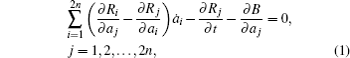
Birkhoffian systems are characterized by the following equations:
which were presented by Birkhoff [ 1 ] and referred to as the Birkhoffian equations by Santilli. [ 2 ] Equation ( 1 ) are clearly a generalization of the Hamiltonian equations since the latter can be recovered from the former as in the particular case of
Therefore, the flow of the Birkhoffian equations shares the similarity of symplecticity preservation with Hamiltonian flows. [ 3 – 5 ] Based on this fact, it is feasible to construct symplectic algorithms for Birkhoffian systems and actually some constructing methods have been presented.
So far, there are mainly two kinds of approaches to construct symplectic algorithms for Birkhoffian systems. One way is to use the generating function method, [ 3 – 6 ] while the other way is based on a direct discretization of the Pfaff–Birkhoff variational principle. [ 7 – 11 ] All resulting algorithms exhibit excellent performance in terms of high accuracy, stability, and preservation of conserved quantities for exceptionally long time. These favorable numerical features, as explained by the backward error analysis, have a close and direct relationship to the structure preservation property. In this article, we propose an indirect method to formulate structure preserving algorithms for Birkhoffian systems. The key of the method is to find a transformation under which the Birkhoffian equations reduce to the Hamiltonian equations. There are many formal symplectic schemes for the Hamiltonian equations, such as the symplectic Euler scheme, the midpoint rule and the Störmer–Verlet method. By applying the corresponding inverse transformation, the image of Hamiltonian symplectic schemes mentioned above can serve as structure preserving algorithms for original Birkhoffian systems.
2. Birkhoffian symplectic algorithms for Birkhoffian systems
As mentioned in the introduction, the flow of the Birkhoffian equations shares the similarity of symplecticity preservation with Hamiltonian flows. If we denote the solution of Eq. ( 1 ) by where a 0 is the initial value of a ( t ) at the initial time t 0 , the symplecticity preservation then means the following algebraic relationship:
Compared with the continuous case, it is natural to define symplectic schemes for Birkhoffian systems. In this paper, we will construct structure preserving algorithms according to the following definition.
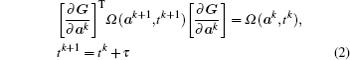
Definition 1 A numerical algorithm applied to Eq. ( 1 ) is called Birkhoffian symplectic, if its step transition map G : a k → a k +1 satisfies
for arbitrary k = 0, 1,…, where τ is the chosen time step. [ 3 ]
Next, we will show how to derive Birkhoffian symplectic algorithms from existing symplectic schemes for Hamiltonian systems. The process mainly relies on the following two propositions.
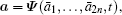
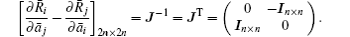
Proposition 1 Suppose that ā = 𝜓 ( a 1 ,…, a 2 n , t ) is an invertible transformation with the inverse the Birkhoffian equations ( 1 ) of variables ( a 1 ,…, a 2 n ) will change into the Hamiltonian equations of variables ( ā 1 ,…, ā 2 n ), if the transformation satisfies
and
for each j = 1, 2,…, 2 n , where Ψ i is the i -th component of .
Proof According to the transformation theory of the Birkhoffian equations, [ 12 ] equation ( 1 ) keeps the form invariant, i.e.,
holds for j = 1,2,…,2 n , if B̄ and R̄ i are chosen as
Note that equation ( 4 ) just means ∂R̄ j / ∂t = 0. Thus, to make Eq. ( 5 ) be the form of the Hamiltonian equations, we only need to set
Direct calculation yields
which implies
Thus, equation ( 3 ) which is the equivalent matrix expression of the above equality is obtained.
Proposition 2 Suppose that the difference scheme ā k +1 = 𝜑( ā k ) is a symplectic algorithm for the Hamiltonian equations i.e.,
𝜓 and are a pair of transformations such that equations ( 3 ) and ( 4 ), then the composite difference scheme will be a Birkhoffian symplectic algorithm for the Birkhoffian equations of variables a .
Proof Identifying a k and ā k as the approximation of a ( t k ) and ā ( t k ), respectively, then we first have the following several equalities:
Thus,
Comparison with Eq. ( 2 ) then completes the proof.
Based on Propositions 1 and 2, the construction of Birkhoffian symplectic algorithms thus comes down to seeking a desirable transformation which fulfills Eqs. ( 3 ) and ( 4 ). One might doubt the existence of the transformation. However, we have the Darboux theorem which guarantees the existence.
Remark 1 Via the transformation which satisfies Eqs. ( 3 ) and ( 4 ), the Birkhoffian equation ( 1 ) are transformed into a Hamiltonian form. The resulting Hamiltonian equations may be canonical or non-autonomous. Anyway, in both cases, it is feasible to construct symplectic algorithms, especially for the canonical Hamiltonian equations. While for the non-autonomous case, by considering the time t as an additional dependent variable and introducing the conjugate momentum h associated with t , the non-autonomous Hamiltonian equations then turn into the canonical case in the extended phase space, and consequently admit symplectic discretization. [ 13 , 14 ] Similar to Proposition 2, Birkhoffian symplectic algorithms can be also derived from symplectic schemes for non-autonomous Hamiltonian systems.
Remark 2 When a practical dynamical system has been given a Birkhoffian representation and furthermore a transformation that fulfills Eqs. ( 3 ) and ( 4 ) has been also found there is no doubt that, the dynamical system automatically admits a Hamiltonian formulation and thus can be directly discretized by symplectic algorithms for Hamiltonian systems. Nonetheless, it does not mean that constructing structure preserving algorithms in the framework of Birkhoffian dynamics is redundant and makes no sense. This is because, for dynamical systems such as the two illustrative examples below, we usually first realize their Birkhoffian representation rather than directly find the Hamiltonian formulation. In the case that the Birkhoffian representation together with a desirable transformation have been found, the developed method then can be used to construct structure preserving algorithms for a practical dynamical system. However, if only the Birkhoffian representation exists but the transformation is hard to be found, this indirect method then fails. In that case, other direct approaches mentioned in the introduction can be employed instead to construct structure preserving algorithms.
3. Illustrative examples
3.1. Linear damped oscillator
Consider the system of a linear damped oscillator
We can give the system a Birkhoffian representation by setting x = a 1 , ẋ = a 2 and taking R 1 = e γt a 2 /2, R 2 = –e γt a 1 /2, and B = e γt ( a 1 2 + a 2 2 + γa 1 a 2 )/2. Namely, the system ( 6 ) has an equivalent expression
Introduce the transformation
then it is trivial to verify that the inverse transformation
satisfies conditions ( 3 ) and ( 4 ) and makes Eq. ( 7 ) change into
which is a Hamiltonian system with the Hamiltonian H = [( ā 1 ) 2 + ( ā 2 ) 2 + γā 1 ā 2 ]/2. As a canonical Hamiltonian system, there are many symplectic algorithms for Eq. ( 8 ). We list three of them here.
Symplectic Euler method
implicit midpoint method
Störmer–Verlet method
Transforming variables ( ā 1 , ā 2 ) back to ( a 1 , a 2 ) then yields
respectively. According to Proposition 2, algorithms ( 9 )–( 11 ) are all Birkhoffian symplectic for Eq. ( 7 ) and consequently for system ( 6 ). In addition, equation ( 10 ) are exactly the structure preserving algorithm formulated in Refs. [ 3 ]–[ 5 ] by the generating function method.
Figure 1 shows numerical solutions and energies of system ( 6 ) obtained by applying algorithms ( 9 )–( 11 ). It is obvious that all of the three Birkhoffian symplectic algorithms simulate the continuous system very well. Since just with first-order accuracy, the method ( 9 ) exhibits a slightly bigger error when simulating the energy compared with algorithms ( 10 ) and ( 11 ). Nonetheless, it still exactly captures the drop of the energy of the system, while traditional methods with the same order accuracy fail, such as the implicit Euler method.
Fig. 1. Numerical solutions (a) and energies (b) of system ( 6 ) corresponding to algorithms ( 9 )–( 11 ).
We are also interested in the preservation of the Birkhoffian B ( a , t ) since for this system it is a conserved quantity. Toward this end, we plot the Birkhoffian versus time, as shown in Fig. 2 . For comparison purpose, the numerical Birkhoffian curve corresponding to the midpoint rule is shown as well. It is obvious that the Birkhoffian associated with the midpoint rule diffuses due to error accumulation, while for Birkhoffian symplectic algorithms, errors of the Birkhoffian always remain bounded. This phenomenon can be understood by realizing that algorithms ( 9 )–( 11 ) are Birkhoffian symplectic for system ( 6 ), but the midpoint rule is not.
Fig. 2. Numerical Birkhoffians (a) of system ( 6 ) and the corresponding errors (b) for algorithms ( 9 – 11 ).
3.2. Single pendulum with linear dissipation
We next consider a single pendulum with linear dissipation
Set θ = a 1 and then the above system admits a Birkhoffian representation with R 1 = e γt a 2 /2, R 2 = –e γt a 1 /2 and B = e γt a 2 2 /2 + γ e γt a 1 a 2 /2 – e γt cos a 1 .
Via the variables transformation
the equivalent Birkhoffian representation reduces to the non-autonomous Hamiltonian equations with the Hamiltonian function As remarked before, there also exists symplectic discretization for non-autonomous Hamiltonian equations, such as the following scheme:
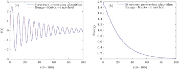
Transforming variables ( ā 1 , ā 2 ) back to ( a 1 , a 2 ) then gives a structure preserving algorithm for the equivalent Birkhoffian representation of system ( 12 ). The numerical solution and energy obtained by applying the structure preserving algorithm are shown in Fig. 3 . Note that the numerical curve obtained by the structure preserving algorithm almost replicates the curve corresponding to the forth order Runge–Kutta method in each graph. It is truly praiseworthy that the structure preserving algorithm nearly performs as well as the forth order Runge–Kutta method, especially when realizing that it only has first-order accuracy.
Fig. 3. Numerical solutions (a) and energies (b) of system ( 12 ) obtained by the structure preserving algorithm and the forth-order Runge–Kutta method, respectively.
4. Conclusion
As the natural generalization of the Hamiltonian equations, the Birkhoffian equations share the similarity of symplecticity preservation. This fact not only serves as the theoretical foundation but also provides an approach to construct symplectic algorithms for Birkhoffian systems. Using the method presented, the construction comes down to seeking a transformation which drives the Birkhoffian equations reduce to the Hamiltonian equations. The Darboux theorem exactly guarantees the existence of the transformation and thus implies that the method is feasible.
Reference
1
Birkhoff G D 1927 Dynamical Systems Providence RI AMS College Publishers
2
Santilli R M 1983 Foundations of Theoretical Mechanics II New York Springer–Verlag


 , Wu Hui-Bin 2 , Mei Feng-Xiang 3 ]