In 1928 Dirac investigated the relativistic wave equation covariance of the Schrodinger equation and proposed a matrix α , β , and relativistic energy to the first order I . ^{[ 1 ]} The Dirac equation describes the motion of a relativistic particle with spin 1/2, which is widely used to solve the problems of nuclear physics and high energy physics. ^{[ 2 ]} One of the important tasks of relativistic quantum mechanics is to find an accurate and exact solution of the Dirac equation for some noncentral physical potentials, which are a mixture of attractive scalar potential S ( r ) and repulsive vector potential V ( r ). Spin symmetry occurs when S ( r ) = V ( r ) and pseudospin (p-spin) symmetry occurs when S ( r ) = − V ( r ). The Dirac equation has been intensively investigated since it has important applications in quantum chemistry and nuclear physics. The Dirac equation is used to describe the motion of particles governed by a strong force when the relativistic effects are taken into account. ^{[ 3 ]}

The Dirac equation for the case of exact spin symmetric occurs when the difference in the magnitude betwen the repulsive vector potential and the attractive scalar potential is zero and the sum of the magnitudes of the repulsive vector potential and attractive scalar potential is equal to a given potential. The exact pseudo-spin symmetry occurs when the sum of the magnitude of the repulsive vector potential and the attractive scalar potential is zero and the difference between the vector potential and scalar potential is equal to a given potential, which is central or non-central. ^{[ 4 ]}

Solutions of the Dirac equation for some typical potentials under special cases of spin symmetry and pseudospin symmetry have been investigated. For spin symmetry κ ( κ + 1) = l ( l + 1) that gives κ = l = j + 1/2 for κ > 0 and κ = −( l + 1) = −( j + 1/2) for κ < 0, where κ is the eigenvalue of the spin orbit coupling operator, l is orbital quantum number, and j is the total angular momentum quantum number. For the pseudospin symmetry case, κ ( κ − 1) = l̃ ( l̃ + 1) that gives κ = l̃ + 1 = j + 1/2 for κ > 0 and κ = − l̃ = −( j + 1/2) for κ < 0, where l̃ is the quantum number of the pseudospin orbital. In nuclear physics, spin symmetry and pseudospin symmetry concepts have been used to study the aspect of deformed and super deformation nuclei. The concept of spin symmetry has been applied to the spectra of meson and antinucleon. ^{[ 5 ]}

Some researchers have investigated the Dirac equation by using a variety of potentials and different methods, such as the spin symmetry in the antinucleon spectrum and tensortype Coulomb potential with spin–orbit number κ in a state of spin symmetry and p-spin symmetry, ^{[ 6 ]} bound states of the Dirac equation with position-dependent mass for the Eckart potential, ^{[ 7 ]} the exact solution of Klein–Gordon with the Pöschl–Teller double-ring-shaped Coulomb potential, ^{[ 8 ]} the exact solution of the Dirac equation for the Coulomb potential plus NAD potential by using the Nikorov–Uvarov method, ^{[ 9 ]} the potential Deng–Fan and the Coulomb potential tensor using the asymptotic iteration method (AIM), ^{[ 10 ]} the potential Poschl–Teller plus the Manning Rosen radial section with the hypergeometry method, ^{[ 11 ]} the solution of Klein–Gordon equation for Hulthen non-central potential in radial part with Romanovski polynomial ^{[ 12 ]} and the solution of the Schrodinger equation with the Hulthen plus Manning– Rosen potential, ^{[ 13 ]} the Scarf potential with the new tensor coupling potential for spin and pseudospin symmetries using Romanovski polynomials, ^{[ 14 ]} for the q-deformed hyperbolic Poschl–Teller potential and the trigonometric Scarf II noncentral potential by using AIM, ^{[ 15 ]} eigensolutions of the deformed Woods–Saxon potential via AIM, ^{[ 16 ]} approximate solutions of the Klein Gordon equation with an improved Manning Rosen potential in D -dimensions using SUSYQM, ^{[ 17 ]} and eigen spectra of the Dirac equation for a deformed Woods–Saxon potential via the similarity transformation. ^{[ 18 ]}

In this study, we will solve the Dirac equation for the Eckart potential plus the trigonometric Manning Rosen potential in a state of spin symmetry using an asymptotic iteration method. The asymptotic iteration method is a method of solving the second-order differential equations. ^{[ 20 ]}

The rest of this paper is organized as follows. The asymptotic iteration method will be briefly reviewed in Section 2. In Section 3, we review the Eckart potential and trigonometric Manning Rosen potential, give a brief introduction to the Dirac equation with equal scalar and vector potentials, and apply the separation of variables in spherical coordinates. In Section 4, we solve the radial and angular parts of the Dirac equation by using the modified Eckart potential combined with trigonometric Manning Rosen potential and obtain the relativistic energy spectrum and wavefunction via the asymptotic iteration method. In Section 5, we present graphically some wavefunctions of the Dirac equation, present several relativistic energy spectra, and discuss some consequences of the results obtained. Finally, some conclusions are drawn from the present study in Section 6.

This method is used to solve differential equation in the following form:

The Dirac equation with scalar potential S ( r ) and vector potential V ( r ) (ℏ = 1, c = 1) is given by

By substituting Eq. ( 24 ) to Eq. ( 11 ), we can immediately obtain two coupled ordinary differential equations for radial parts of Dirac eigen functions as follows:

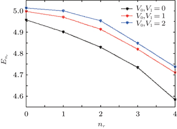
In this section, we discuss several results obtained in the previous section. From the energy eigen value in Eq. ( 41 ) and the orbital quantum number in Eq. ( 52 ), by using Matlab, we have the numeric solution of the energy eigen value, and the results are listed in Table  1 with parameters v = 0.25, α = 0.5, V ₀ = 0.4, V ₁ = 0.6, and M = 5 fm ⁻¹ . The positive value is taken due to the spin symmetric limit. Table  1 shows that the increases of values q and n _r in the same quantum state cause the energy eigenvalue to decrease.

Table 1.

Table 1.

Table 1. Energy eigenvalues corresponding to several states of a particle under the influence of the Eckart potential and trigonometric Manning Rosen potential. . n r n l m E n r n lm /fm −1 q = 0.2 fm −1 q = 0.1 fm −1 q = 0.04 fm −1 1 0 0 4.9733 4.9921 4.9989 1 1 0 4.9491 4.9845 4.9984 1 1 1 4.9405 4.9831 4.9981 1 2 0 4.9148 4.9753 4.9976 2 0 0 4.9362 4.9816 4.9968 2 1 0 4.8998 4.9689 4.9962 2 1 1 4.8878 4.9568 4.9954 2 2 0 4.8531 4.9531 4.9949

Table 1. Energy eigenvalues corresponding to several states of a particle under the influence of the Eckart potential and trigonometric Manning Rosen potential. .

Table  2 lists the energy eigen values with different values of potential constant V ₀ and V ₁ , which are plotted in Fig.  1 for different values of V ₀ and V ₁ . Figure  1 shows that the increases of potential constant V ₀ and V ₁ cause the energy to decrease.

Table 2.

Table 2.

Table 2. Energy eigenvalues (in fm −1 ) with M = 5; C = 5; v = 0.25; q = 0.2; α = 0.5, for a particle under the influences of the Eckart potential and the trigonometric Manning Rosen potential V 0 and V 1 . . n l M V 0 V 1 E 0 E 1 E 2 E 3 E 4 2 2 0 0 4,9579 4,9014 4,8287 4,7348 4.5837 2 2 1 1 4,9976 4,9701 4,9136 4,8202 4,7105 2 2 2 2 5,0131 4,9999 4,9535 4,8484 4,7379

Table 2. Energy eigenvalues (in fm −1 ) with M = 5; C = 5; v = 0.25; q = 0.2; α = 0.5, for a particle under the influences of the Eckart potential and the trigonometric Manning Rosen potential V 0 and V 1 . .

Fig. 1.

	Figure Option View Download New Window
	Fig. 1. Energy eigenvalues for different values of V 0 and V 1 .

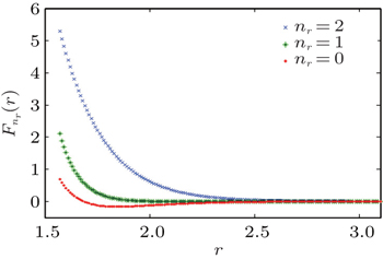
By varying parameters corresponding to values of δ and γ , some of the radial wavefunctions are listed in Table  3 . Radial wavefunctions for a particle under the influences of the Eckart potential and the trigonometric Manning Rosen potential are affected by potential constants V ₀ and V ₁ , and by parameter q as well. The parameter q has a dimension of inversed distance in space, which describes the effect range of the trigonometric Manning Rosen potential in space. If q is enlarged, it physically means that the potential range is smaller in a space. Table  3 and figure  2 show that the variation of n _r for the radial wavefunction induces the distribution of particles to move away from or approach to the core of the atom. From Fig.  2 it follows that amplitude n _r = 1 < n _r = 2, which means that at n _r = 2, the distribution of particles moves away from the nucleus compared with the case of smaller n _r . This indicates that the higher the value of n _r is, the greater the distance of the particle from the core is.

Table 3.

Table 3.

Table 3. Energy eigenvalues (in fm −1 ) with M = 5, C = 5, n l = 2, m = 2, v = 0.25, V 0 = 2, V 2 = 2, q = 0.2, α = 0.5, for a particle under the influences of the Eckart potential and the trigonometric Manning Rosen potential variation n r . . n r E n r F n r 0 5.0131 1 4.9999 2 4.9535

Table 3. Energy eigenvalues (in fm −1 ) with M = 5, C = 5, n l = 2, m = 2, v = 0.25, V 0 = 2, V 2 = 2, q = 0.2, α = 0.5, for a particle under the influences of the Eckart potential and the trigonometric Manning Rosen potential variation n r . .

Fig. 2.

	Figure Option View Download New Window
	Fig. 2. Radial wavefunction from Table  3 for different values of n r .

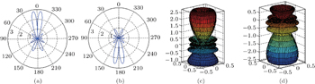
For the angular solution of the wavefunction in Eq. ( 54 ), we compare two spinor wavefunctions with the same angular quantum number n _l = 4 but different values of α and β which corespond to parameters V ₀ and V ₁ in Fig.  3 . The plots are displayed in two and three dimensions together with the wave function. In Figs.  3(a) and 3(b) , α < β ; in Figs.  3(c) and 3(d) , α > β . For the same value of n _l , the sum of waves does not change.

Fig. 3.

Figure Option View Download New Window

Fig. 3. (a), (b) Two-dimensional and (c), (d) three-dimensional representations of the anglar wave function for a state n l = 4. In panels (a) and (b), Q ( θ ) = 1.57638(1.5865 + 16.793(−1 + cos( θ )) + 42.105(−1 + cos( θ )) 2 + 36.695(−1 + cos( θ )) 3 + 10.215(−1 + cos( θ )) 4 ) 2 (1−cos( θ )) 0.2 (1 + cos( θ )) 1.16 ; in panels (c) and (d), ( θ ) = 1.57638(6.7983 + 39.2793(−1 + cos( θ )) + 67.9901(−1 + cos( θ )) 2 + 45.3199(−1 + cos( θ )) 3 + 10.2495(−1 + cos( θ )) 4 ) 2 (1−cos( θ )) 1.4 (1 + cos( θ )) 0.27 .

Fig. 4.

	Figure Option View Download New Window
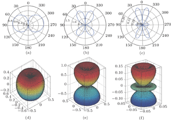
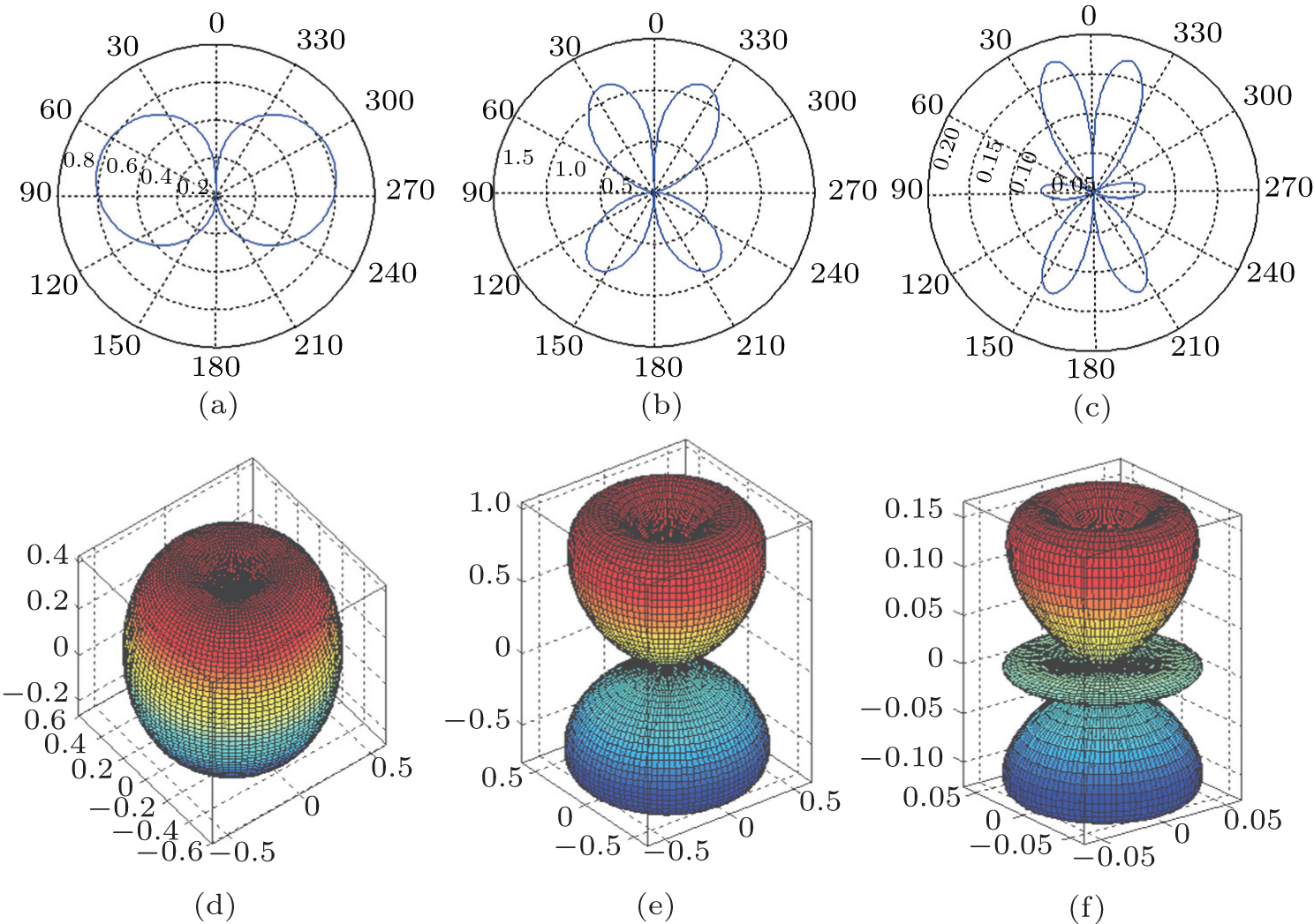	Fig. 4. (a), (c) Polar diagrams and (d), (f) three-dimensional anguler wavefunctions with n l = 0 (a), (d), 1 (b), (e), and 2 (c), (f).

In this paper, we study the Dirac equation for particle spin-1/2 in the Eckart potential combined with the trigonometric Manning Rosen potential in condition that the scalar potential equals the vector potential. The radial part of the spinor wavefunction is obtained approximately from Eq. ( 44 ) and the angular part from Eq. ( 54 ). The results show that the disturbances of the Eckart and trigonometric Manning Rosen potentials change the radial part and the angular part of the wavefunction. The energy eigenvalue can be obtained via the asymptotic iteration method in Eq. ( 41 ) and the equation of orbital quantum number l as expressed in Eq. ( 52 ), where both are interrelated between quantum numbers. The energy spectrum is also numerically solved using Matlab software, showing that the increase of the radial quantum number n _r causes the energy to decrease.