

A new traffic model with a lane-changing viscosity term
[Ko Hung-Tang, Liu Xiao-He, Guo Ming-Min† , Wu Zheng]
, Wu Zheng]
|
|


†Corresponding author. E-mail: mmguo@fudan.edu.cn
*Project supported by the National Natural Science Foundation of China (Grant Nos. 11002035 and 11372147) and Hui-Chun Chin and Tsung-Dao Lee Chinese Undergraduate Research Endowment (Grant No. CURE 14024).
In this paper, a new continuum traffic flow model is proposed, with a lane-changing source term in the continuity equation and a lane-changing viscosity term in the acceleration equation. Based on previous literature, the source term addresses the impact of speed difference and density difference between adjacent lanes, which provides better precision for free lane-changing simulation; the viscosity term turns lane-changing behavior to a “force” that may influence speed distribution. Using a flux-splitting scheme for the model discretization, two cases are investigated numerically. The case under a homogeneous initial condition shows that the numerical results by our model agree well with the analytical ones; the case with a small initial disturbance shows that our model can simulate the evolution of perturbation, including propagation, dissipation, cluster effect and stop-and-go phenomenon.
The continuum model is an effective tool for traffic flow analysis with a history of more than half a century. Early in 1955, Lighthill and Whitham, [1] and Richards, [2] respectively originated this model by applying the continuity equation in fluid mechanics to traffic flow on a long freeway, known as the LWR theory. In the 1970s, Payne built a second-order continuum traffic model with an acceleration equation based on carfollowing theory, which can be likened to the one-dimensional (1D) Navier– Stokes equation.[3] Payne also presented a difference scheme for his model, which makes using a numerical computation method to study traffic flow possible.[4] Other models were developed based on Payne’ s model, [5, 6] with viscosity terms involving the speed or density gradient on a single lane. However, such models did not consider the impact of traffic conditions on adjacent lanes and lane-changing behavior.
The lane-changing problem has received increasing scientific attention in the last decade, and is still a thorny problem. According to the reviews by Zheng, [7] Moridpour et al., [8] and Toledo, [9] lane-changing models are categorized into two groups: LCI (lane changing impact) models aiming to quantify the impact of lane-changing behavior on surrounding vehicles; LCD (lane changing decision) models aiming to capture the lane changing decision-making process. Comparatively, LCD models are studied more thoroughly than LCI models. Meanwhile, the previous LCI models focused on the impact of lanechanging behavior only on the continuity equation, while its impact on the acceleration equation still remains unexplored.
In the LCI models of Zhu et al., [10, 11] Laval et al., [12] Jin, [13] and Sun et al., [14] source terms were added to the continuity equation to simulate the impact of lane-changing. In Zhu’ s model, the source term involves the density difference between adjacent lanes, while in Laval’ s model, it is the speed difference between adjacent lanes that affects the source term; these two source terms may lead to different equilibrium states (to be discussed later in this paper). In Jin’ s model, LC intensity was introduced to quantify the lane-changing behavior, which is another form of source term. However, this makes the conservation of total vehicle number very hard to verify. In Sun’ s model, not only a source term was added to the continuity equation, but also a viscosity term was added to the acceleration equation. Notably, this viscosity term has no direct relationship with lane-changing behavior.
Usually, drivers change lanes to pursue a more comfortable driving environment or a faster speed (free lanechanging). When some vehicles on a slow lane change to a faster lane, the density of the faster lane increases and thus its speed reduces, and the speed of the slower lane increases due to the decrease of its density. Therefore, lane-changing causes both density difference and speed difference between adjacent lanes to decrease. This is analogous to the viscosity of Newtonian fluids, where a tangential stress induced by the speed gradient of adjacent flow layers drives the flow to reach a new equilibrium state. Similar to the Navier– Stokes equation of viscous flow, in this paper, we add a viscosity term related to the speed difference and density difference on y direction (perpendicular to the direction of traffic flow, that is, x direction) to the acceleration equation, so as to simulate the impact of lane-changing behavior on traffic flow.
The remainder of this paper is organized as follows. In Section 2, a new continuum traffic model with a lane-changing viscosity term is introduced and explained. In Section 3, a numerical discretization method of this model is given. Numerical results are presented in Section 4, where the reliability of this model is shown and the simulation results of perturbation’ s evolution are discussed. Finally, a conclusion is drawn in Section 5.
Due to the changes of vehicle number on each lane caused by lane-changing, a source term is needed to add to the continuum equation. Furthermore, we introduce a “ viscous force” term to the original acceleration equation of Payne’ s model to demonstrate the impact of lane-changing on traffic flow dynamics. The general form of this model is
where ρ l and ql are the vehicle density and flow rate on the l-th lane, respectively; a and Tr are the sonic speed and time delay; Qe (ρ ) = ρ Ue (ρ ), Ue (ρ ) is the equilibrium speed function; Φ l′ l is the net lane-changing rate, which equals to the rate of vehicles that change from the l′ -th lane to the l-th lane minus the rate of vehicles that change from the l-th lane to the l′ -th lane per hour per kilometer; fviscous, l is the “ viscous force” per unit length, with a unit of veh· h− 2. In this paper, free flow speed is denoted by uf; jam density is denoted by ρ j.
In Laval’ s model, the source term Φ l′ l is based on the speed difference Δ ul′ l between adjacent lanes. Suppose Δ ul′ l = ul − ul′ > 0, then Φ l′ l is determined as follows:


where τ is a constant parameter; Δ t and Δ x are temporal step and spatial step, respectively, assuming Δ x /Δ t = uf; Q is the maximum flow rate. Laval' s model consists of the first equation of Eq. (1) and a triangular fundamental diagram instead of the acceleration equation

where w is the congestion wave speed (w ≈ uf/4). We derive from this equation that Q ≈ ρ juf / 5. Rearrange Eqs. (2)– (5), a simplified form of source term can be obtained as follows:

In Zhu’ s model, [10, 11] another form of source term based on density difference between adjacent lanes is used. This form is simpler but discontinuous

where kl′ l is a constant. To avoid the computation inconvenience caused by discontinuity, we can simplify Zhu’ s source term according to the simplification of Laval’ s source term. Suppose the density difference Δ ρ l′ l = ρ l′ − ρ l > 0, then

The source terms of Laval’ s model and Zhu’ s model emphasized the differences between adjacent lanes, so both models can simulate well the phenomenon of density equalization in the lane-changing problem. However, they both have weaknesses. Laval’ s model cannot cover car-following phenomenon since it is a single-equation model, and Zhu’ s model does not include a “ viscous force” term driven by lanechanging to its acceleration equation, which is incomplete for lane-changing simulation. Besides, as the source terms are determined by either speed difference or density difference in both models, lane-changing behavior stops happening when speed difference is zero or density difference is zero, which means Laval’ s model implies an equilibrium state when adjacent lanes have the same speed but different densities, while Zhu’ s model implies an equilibrium state when adjacent lanes have the same density but different speeds. This contradicts real traffic phenomenon. In order to avoid these weaknesses, we combine Eqs. (7) and (9), and introduce a new source term that considers both speed difference and density difference between adjacent lanes


where C1 and C2 are dimensional constants, C1 has a unit of h· km− 2, and C2 has a unit of km· h− 1· veh− 1.
The form of “ viscous force” fviscous, l in Eq. (1) can be obtained as follows: Given that fviscous, l is driven by the difference between adjacent lanes, we may assume an ideal state where the traffic condition is homogenous in each lane, that is, all terms of partial derivatives with respect to x equal to zero and traffic flow is close to the equilibrium state. Therefore, the term of equilibrium speed function can be dropped. Thus equation (1) is simplified to
Applying the triangular fundamental diagram (6), we obtain

Note that fviscous, l is a function of Φ l′ l, which can be easily determined by Eqs. (10)– (12).
Now the control equations of our new model are fully developed as follows:
where the lane changing source term demonstrates the impact of speed difference and density difference between adjacent lanes on free lane-changing behavior, and the viscosity term addresses the momentum exchange induced by the lane-changing behavior. Other factors that may influence lanechanging behaviors in real traffic situations can be added to the proposed model.
Let L be the characteristic length, and let q* = q/Q, u* = u/uf, ρ * = ρ /ρ j, x* = x/L, t* = t/(L / uf), a* = a/uf, Tr* = Tr/(L / uf), 

Accordingly, equations (11), (12), and (14) change to


where

The ranges of values of C1 and C2 were estimated according to the empirical traffic data from an 81-meter long section on Yan’ an Elevated Road, Shanghai, China. The data were extracted from a video recorded on July 21, 2008, from 7:40 a.m. to 11:00 a.m. and were grouped every ten minutes, including density and speed on each lane, and the number of lane-changing to the left (this can be regarded as free lanechanging, in contrast to compulsive lane-changing, for example, lane changing to the right triggered by a ramp ahead). Density and speed were calculated according to the coordinates of vehicles on each video frame.[15, 16] The number of lane changes was manually counted from the video.
We determined the upper limits of C1 and C2 through data fitting. Generally, we have C1 ≤ 0.3 h· km− 2 and C2 ≤ 25 km· h− 1· veh− 1, and dimensionless parameters 

We use an explicit flux vector splitting scheme of finitedifference methods to discretize the model equations. Rewrite Eq. (14) as

where

and

which are all 2l-dimensional vectors (l is the total number of lanes, different from its definition in Section 2). Define Jacobi matrix as A = ∂ f/∂ u. Apparently, f = Au; thus the requirement for the flux vector splitting scheme is satisfied.
For computation, firstly, split the flux vector. Rewrite the matrix A to A = Φ Λ Φ − 1, where Λ is the eigenvalue matrix and Φ is the eigenvector matrix. Let Λ + = (Λ + | Λ | ) / 2, Λ − = Λ − Λ + , then we have the positive flux vector f+ = Φ Λ + Φ − 1u and the negative flux vector f− = Φ Λ − Φ − 1u.
Secondly, calculate the source term according to Eqs. (17)– (20).
Thirdly, advance time steps according to the following equation:

Since this scheme is conservative, and considers the characteristics of hyperbolic equation, it can provide precise results for the direction and wave speed of perturbation propagation.
The linear stability condition of this scheme is obtained, which is

Obviously, this stability condition agrees with the CFL condition, which requires the numerical domain of dependence of any grid point to include the analytical domain of dependence.
In order to validate the new model and the discretization scheme, we study a simple two-lane situation: lane 1 is the fast lane with lower density; lane 2 is the slow lane with higher density; speed and density on both lanes are evenly distributed, so variables will not change with respect to x direction. Hence, the dimensionless control equations are simplified as follows:

where lane-changing function
equilibrium flow Qe (ρ ) = 5ρ (1 − ρ ), and the initial values are ρ 10, ρ 20, q10, and q20, respectively. The characteristic values are set as L = 15 km, uf = 90 km· h− 1, ρ j = 143 veh· km− 1 (the same as that in Section 4.2). Equation (23) is ordinary differential equations. Its accurate results can be achieved through the fourth-order Runge– Kutta method, which will be regarded as analytical results hereafter.
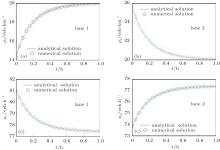
Numerical results and analytical results are shown in Figs. 1 and 2 (with the dimensional units indicated on the axes). Numerical results are obtained as described in Section 3. Constants are set as Tr = 0.02, a = 0.4, C1 = 0.25,
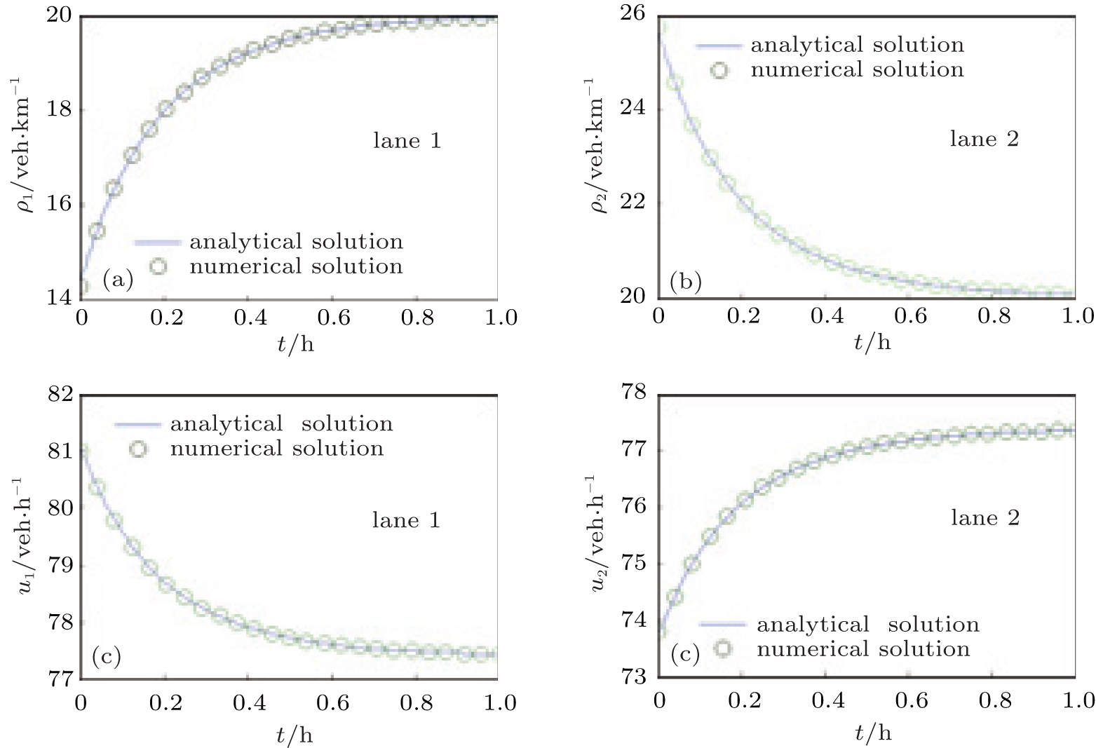 | Fig. 1. Numerical results against analytical results at low density (ρ 10 = 14.3 veh· km− 1, ρ 20 = 25.74 veh· km− 1). (a) Density evolution in lane 1, (b) density evolution in lane 2, (c) speed evolution in lane 1, and (d) speed evolution in lane 2. |
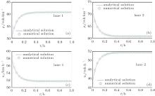
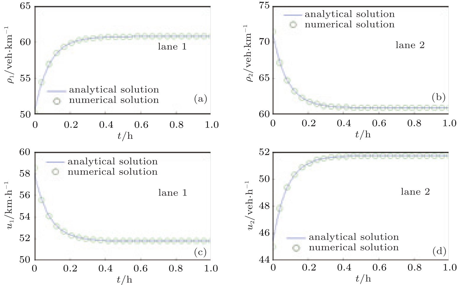 | Fig. 2. Numerical results against analytical results at medium density (ρ 10 = 50.05 veh· km− 1, ρ 20 = 71.5 veh· km− 1). (a) Density evolution in lane 1, (b) density evolution in lane 2, (c) speed evolution in lane 1, and (d) speed evolution in lane 2. |
C2 = 1.5, Δ x = 0.1, and Δ t = 0.01; in Fig. 1, ρ 10 = 0.1, ρ 20 = 0.18, q10 = 0.9, and q20 = 0.82; in Fig. 2, ρ 10 = 0.35, ρ 20 = 0.5, q10 = 0.65, and q20 = 0.5. Note that the values adopted for C1 and C2 in this case are half of the upper limits determined in Section 2.3, which indicates that this case is assumed to have a medium lane changing intensity.
It is shown in this case that our model simulates the traffic with lane-changing behavior accurately both at low density and at medium density (similar results can be achieved for higher density). In Figs. 1 and 2, speed and density of the two lanes differ at the beginning, then monotonically converge towards each other, and reach an equilibrium state at last, which agrees with the real traffic process. It is also shown that the discretization scheme adopted ensures the convergence of the numerical method, because the numerical results agree with the analytical results not only in quality, but also in quantity, and they require the same amount of time to reach the equilibrium state.
Perturbation’ s evolution has been an important problem for the study of traffic models. Arising from perturbation problems, cluster effect is a typical phenomenon in nonlinear systems, as suggested by Kerner[16] and Sun et al.[14] We explored this problem using the same initial condition of small perturbation in density as adopted by Kerner and Sun et al.
Initial flow is the product of density and equilibrium speed, and the equilibrium speed is adopted from Ref. [17]
We use homogeneous Neumann boundary conditions at upstream and downstream, the discretization of which is

where J is the total grid number in x direction. Constants are set to Tr = 0.02, a = 0.4, C1 = 0.25, C2 = 1.5, Δ x = 0.01, and Δ t = 0.002.
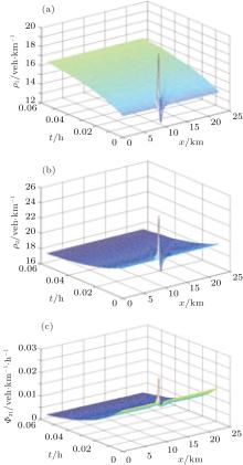
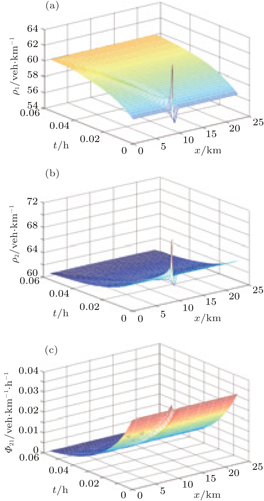
First, for the low-density situation, we set ρ 10 = 0.1 and ρ 20 = 0.14. Results are shown in Fig. 3. Perturbation propagates to downstream and then dissipates.
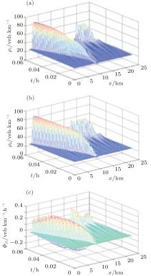
Then, we change the initial condition of lane 2 to medium-density, and set ρ 10 = 0.1 and ρ 20 = 0.21. Results show that without lane-changing terms, perturbation in lane 2 leads to congestion both upstream and downstream. However, results of our lane-changing model (Fig. 4) show that in lane 2, although breakdown still happens upstream, congestion does not appear downstream. Instead, lane-changing happens frequently, resulting in a gradual increase of the density at downstream in lane 1 and a cluster appearing in lane 2. Therefore, lane-changing behavior alleviates the traffic congestion.
 | Fig. 3. Dissipation of perturbation at low-density. (a) and (b) Density evolutions in lane 1 and lane 2, respectively. (c) The evolution of non-dimensional net lanechanging rate from lane 2 to lane 1. |
When changing the initial condition of lane 1 to mediumdensity as well, that is, ρ 10 = 0.19 and ρ 20 = 0.21, we found that its ability to alleviate congestion reduces (Fig. 5), and perturbation turns to several clusters with different speeds in both lanes, which results in a stop-and-go wave. The net lanechanging rate profile also shows that, in this state, there are more vehicles that change lanes from lane 1 to lane 2 than their counterparts in front of the congestion wave. This phenomenon can also be observed in real traffic.
Finally, we change the initial conditions of both lanes to high-density, that is, ρ 10 = 0.4 and ρ 20 = 0.45. A perturbation wave propagates to upstream and dissipates shortly after, as shown in Fig. 6.
Our results are consistent with Kerner’ s simulations.[17] However, they combined several lanes to one lane, whereas our viscous lane-changing model can provide the detailed evolution of perturbation on each lane. It is proved in this case
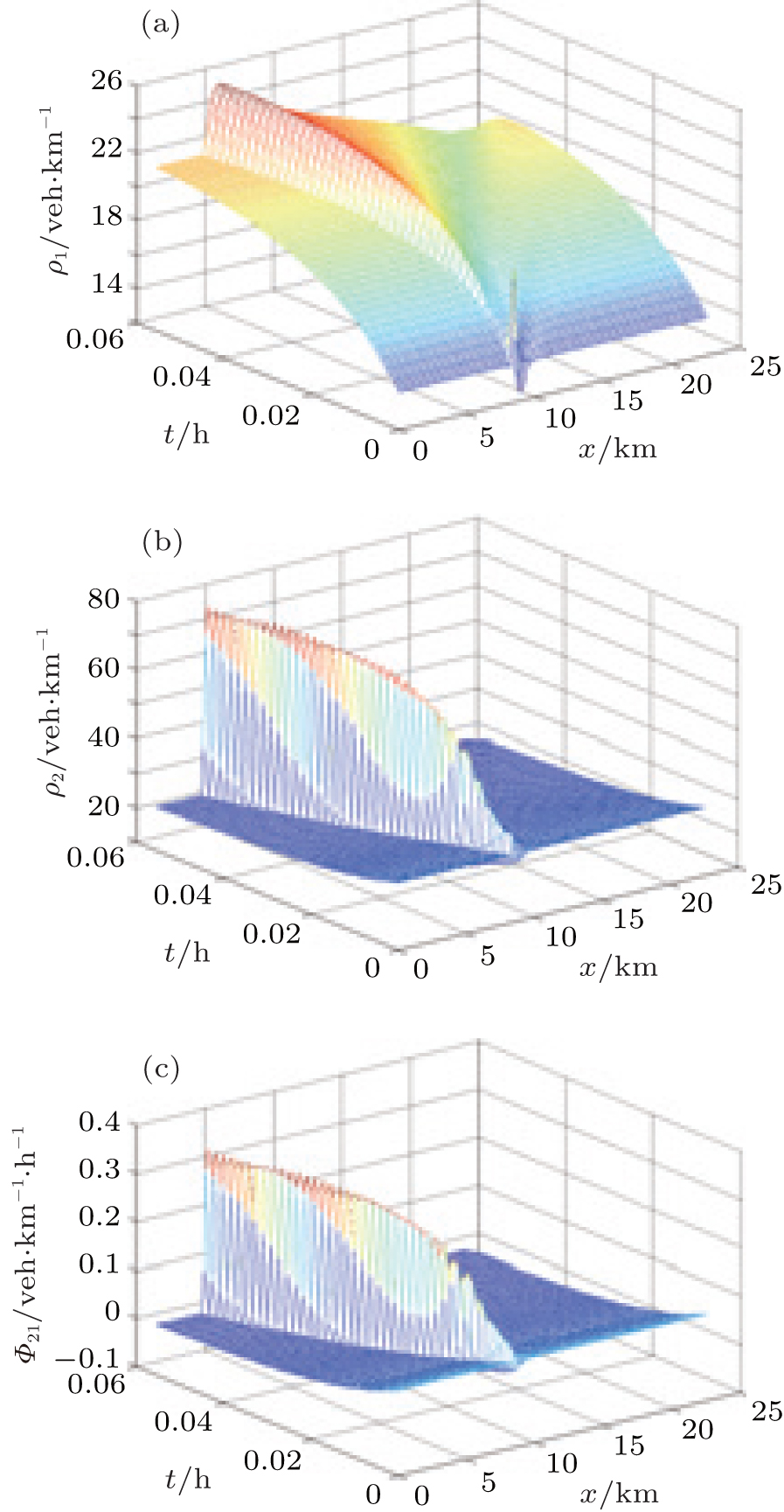 | Fig. 4. Medium-density in lane 2 and low-density in lane 1. (a) and (b) Density evolutions in lane 1 and lane 2, respectively. (c) The evolution of non-dimensional net lane-changing rate from lane 2 to lane 1. |
that lane-changing behavior helps to alleviate congestion. In Fig. 4, without lane-changing terms, lane 2 is congested while lane 1 remains clear; with lane-changing terms, both lanes are not congested. This conclusion agrees with real traffic phenomenon.
In this paper we established a new traffic flow model by adding a lane-changing source term and a lane-changing viscosity term to Payne’ s model. This model focused on two types of impact on traffic flow by lane-changing behavior: the equalization of speed and density. We explored two cases considering lane-changing and car-following; our results are similar to Kerner’ s results that only consider the car-following effect, but our model is better because it provides the traffic state of each individual lane with details.
The proposed model is designed for free lane-changing
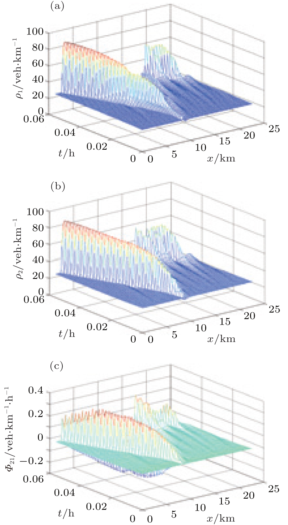 | Fig. 5. Stop-and-go wave at medium-density. (a) and (b) Density evolutions in lane 1 and lane 2, respectively. (c) The evolution of non-dimensional net lane-changing rate from lane 2 to lane 1. |
 | Fig. 6. Dissipation of perturbation at high-density. (a) and (b) Density evolutions in lane 1 and lane 2, respectively. (c) The evolution of non-dimensional net lane-changing rate from lane 2 to lane 1. |
problems, where drivers change lanes to move faster or to move in a less crowded environment. Compulsive lanechanging problems, where traffic rules and drivers’ destination have impact on lane-changing behavior, may be explored in the future based on this model.
| 1 |
|
| 2 |
|
| 3 |
|
| 4 |
|
| 5 |
|
| 6 |
|
| 7 |
|
| 8 |
|
| 9 |
|
| 10 |
|
| 11 |
|
| 12 |
|
| 13 |
|
| 14 |
|
| 15 |
|
| 16 |
|
| 17 |
|