The magnetization dynamics of nanoscale magnetic structures have attracted considerable attention, both for fundamental reasons and because of their potential technological applications.^{[1– 10]} Over last few years, the dynamic properties of patterned magnetic elements with various shapes and sizes have been studied extensively.^{[11– 14]} Several new features, such as localization and quantization of the spin-wave modes, have been discovered and characterized. For example, in uniformly magnetized rectangular or elliptical elements, the spin wave spectrum exhibits discrete eigenfrequencies.^{[15, 16]} The lowest spin-wave mode is the edge mode which is localized near the element edges due to the strong inhomogeneity in the internal magnetic field at the edges. Above the uniform resonance frequency, a series of quantized spin waves are found, which are related to the lateral confinement.

An understanding of the dynamic properties of nanoscale magnets is also necessary for their application. The magnetization reversal has a close relation with dynamic properties of magnets.^{[17– 20]} It is found that the occurrence of reversal is always accompanied by the softening of one of the spin-wave modes (its frequency goes to zero at switching field) and the spatial behavior of softening mode determines the reversal process.^[21] In rectangular elements, the reversal is initiated by the softening of the edge mode and is completed by the nucleation of reversed domain and its succedent irreversible expansion through the domain wall movement.^{[22, 23]} If the ends of the rectangular elements are tapered, then it is the softening of the fundamental mode that triggers the reversal and a uniform rotation process is realized.^[24] The speed of reversal depends on whether it occurs by coherent rotation or by the generation of several nonuniform modes. The structures with tapered ends have been suggested as a way to eliminate the influence of edge effect and to promote fast, ordered uniform switching, making it attractive for use as a magnetic memory element.^{[22– 24]} Moreover, by exciting a certain spin-wave mode, one can not only reduce the switching field greatly but also choose a desirable reversal process.^{[25– 28]} Therefore, in order to obtain a required magnetization reversal, it is necessary to study the spectral and spatial characteristics of spin-wave modes in nanoscale magnets, and especially to manipulate them as required.

In this paper, by using micromagnetic simulations, we study the dynamic properties of magnetic nanoelements and their manipulation by changing the element shape. The spectra and spatial distributions of the spin-wave modes and their evolution with the shape are obtained and explained.

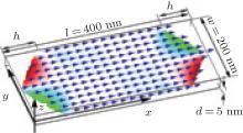
Micromagnetic simulation is an important method to study the dynamic properties of nanomagnets. Its validity has been demonstrated by many experiments. The magnetic nanoelement with tapered ends used in the simulations is 400 nm long in the x direction, 200 nm wide in the y direction, and 5 nm thick in the z direction, as shown in Fig. 1. The tapered degree of the nanoelement is represented by h, which changes from 0 to 200 nm. The magnetic parameters corresponding to Permalloy are chosen in micromagnetic simulations: saturation magnetization M_s = 8.6 × 10⁵ A/m, exchange stiffness A_ex = 1.3× 10^{− 11} J/m, and magnetocrystalline anisotropy K = 0. The simulations presented here are performed using object oriented micromagnetic framework (OOMMF) through solving the Landau– Lifshitz– Gilbert (LLG) equation.^[29] The simulation cell size is chosen to be 2× 2× 5 nm³. The equilibrium magnetization state of the elements is reached by relaxing an initial uniform magnetization state under a constant external field (H_app= 100 mT) pointing to the x direction. As an example, the equilibrium state for h= 40 nm is shown in Fig. 1. The magnetization is parallel to external magnetic field except for the edges, where magnetization tends to lie parallel to the lateral sides to reduce stray field. The spin waves are excited by a short out-of-plane (z direction) rectangular magnetic pulse field with an amplitude of 0.1 mT and a pulse duration τ = 0.3 ns. In order to excite many more spin wave modes, except the uniform field pulse (UNI), the anti-symmetric pulses (AS-x and AS-y) with respect to the x axis and y axis are used. The time evolution of the magnetization for each cell is recorded at a regular time interval of 5 ps. The local power spectrum from each cell is obtained by performing a Fourier analysis on the component of the magnetization perpendicular to the film surface. The overall power spectrum, with a frequency resolution of 0.05 GHz, is obtained by summing the local power spectra over the whole element. The spatial distribution of spin-wave eigenmode is imaged by plotting the oscillation amplitude of each cell at the given frequency.

Fig. 1.

	Figure Option ViewDownloadNew Window
	Fig. 1. Illustration of the tapered nanoelement with the geometry and dimensions. The arrows represent the magnetization vectors in the equilibrium state under applied magnetic field Happ = 100 mT.

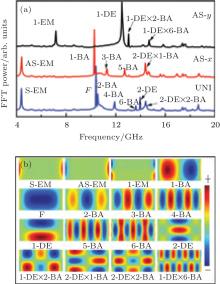
The spin-wave resonance frequency spectra of the rectangle shape (h= 0 nm) are shown in Fig. 2(a). It can be seen that several distinct resonance peaks are excited, corresponding to different spin-wave normal modes. The spatial distributions of each normal mode FFT power are imaged in Fig. 2(b). The spin-wave modes can be classified following the spatial distribution of dynamic magnetization as used in Ref. [15]. The lowest frequency modes are edge modes labeled as EM, which are localized at the edge of the element. Two kinds of edge modes are excited, 1-EM and degenerate 0-EM modes (labeled as S-EM and AS-EM). The second lowest frequency mode is the fundamental mode (labeled as the F mode), whose oscillation concentrates in the central area of the element and is similar to the Kittel uniform mode detected in a ferromagnetic resonance experiment (FMR).^[30] The n-BA modes are standing-wave modes with nodes parallel to the static magnetization labeled. These modes resemble the backward modes of spin waves in films. The last two kinds of modes are m-DE standing spin-wave modes, whose nodes are lined in the direction perpendicular to the static magnetization resembling the Damon– Eshbach (DE) mode of continuous films, and the mixed standing-wave modes n-BA× m-DE. It is worth mentioning that all of the spin-wave modes excited by the uniform pulse field are symmetric in the x and y directions, meaning that only the standing-wave modes with even n and m or the modes having the same phase (F and S-EM modes) can be excited. If the AS-x (or AS-y) pulse field is used, only antisymmetric AS-EM mode and n-BA modes with odd n (or m-DE modes with odd m) are excited. The symmetry of the spin-wave mode is determined by the symmetry of the exciting force.

Fig. 2.

	Figure Option ViewDownloadNew Window
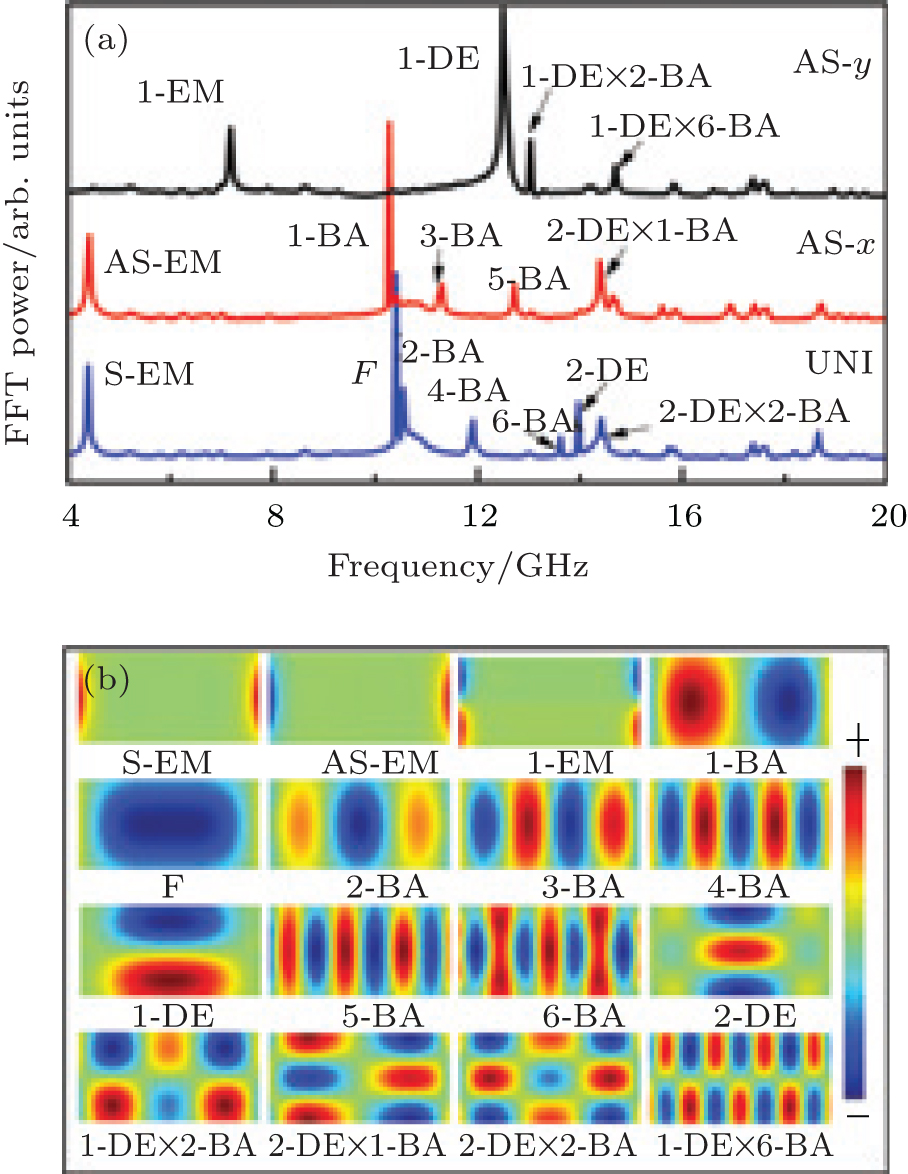	Fig. 2. (a) Spin-wave resonance frequency spectra of the rectangle element excited by uniform pulse (UNI), x antisymmetric pulse (AS-x) and y antisymmetric pulse (AS-y). (b) Spatial distributions of the FFT power of the spin-wave modes for the rectangular element.

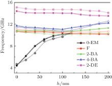
The influence of the element shape on the spin-wave modes can be clearly observed from Figs. 3(a) and 3(b), where the frequency spectra and the mode spatial behavior for the tapered elements with different h excited by the uniform pulse field are shown. The most influenced mode is the edge mode, whose frequency increases rapidly with the tapered degree h. When h ≥ 100 nm, the resonance peak of edge mode is merged with the fundamental mode. Other normal modes are much less affected by the tapered end of the element. The shifts of the frequencies for these modes are small and they display different tendencies. For F and 2-DE modes, the frequency decreases slightly with the increase of h. However, for 2-BA and 4-BA modes, the frequency decreases at first and then increases with the increase of h. The influence of the element shape on the spin wave normal modes is also exhibited on the spatial distributions of the mode FFT power, as shown in Fig. 3(b); where, as an example, the power spatial profiles and their evolutions with the tapered degree h for edge mode and fundamental mode are depicted. It can be seen that with the increase of h, the oscillation areas of the edge mode in both ends of the element gradually increase and move toward the central area. When h> 100 nm, they merge into the fundamental mode completely. In other words, the edge mode disappears. Moreover, the degeneracy of the edge modes are gradually lifted when h> 60 nm, which is clearly revealed in Fig. 3(c). The frequency of in-phase edge mode S-EM is a little higher than that of the out-of-phase mode AS-EM and the frequency difference increases gradually with h. The lift of the edge mode degeneracy is due to the dynamic dipolar interaction between the left and right parts of the mode. As mentioned above, with the increase of the parameter h, the edge mode gradually moves toward the central area. This gives rise to the increase of the dynamic dipolar interaction, leading to the split of the degenerate edge modes. The shape- or size-induced frequency split of mode was recently observed in Brillouin light scattering measurements.^{[31, 32]} It is worth noting that the main results still hold true for other nanoelements with different sizes and aspect ratios.

It is widely recognized that the quantization and localization of spin waves in nanomagnets come from the lateral confinement and the confinement-induced strong inhomogeneity of the internal magnetic field, even in a homogeneously magnetized sample.^{[15, 33, 34]} When a spin wave propagates in a region with strong inhomogeneous internal field, its wave vector k is a function of position. At a point where k becomes complex number, the spin wave will be reflected. Therefore, the spin wave is confined in an area where k can only be a real number. This is the so-called “ spin-wave well” .^{[35, 36]} When spin waves can propagate through the magnet, the spatial lateral confinement of nanomagnet gives rise to the quantization of the spin waves, forming standing-wave modes.

Fig. 3.

Figure Option ViewDownloadNew Window

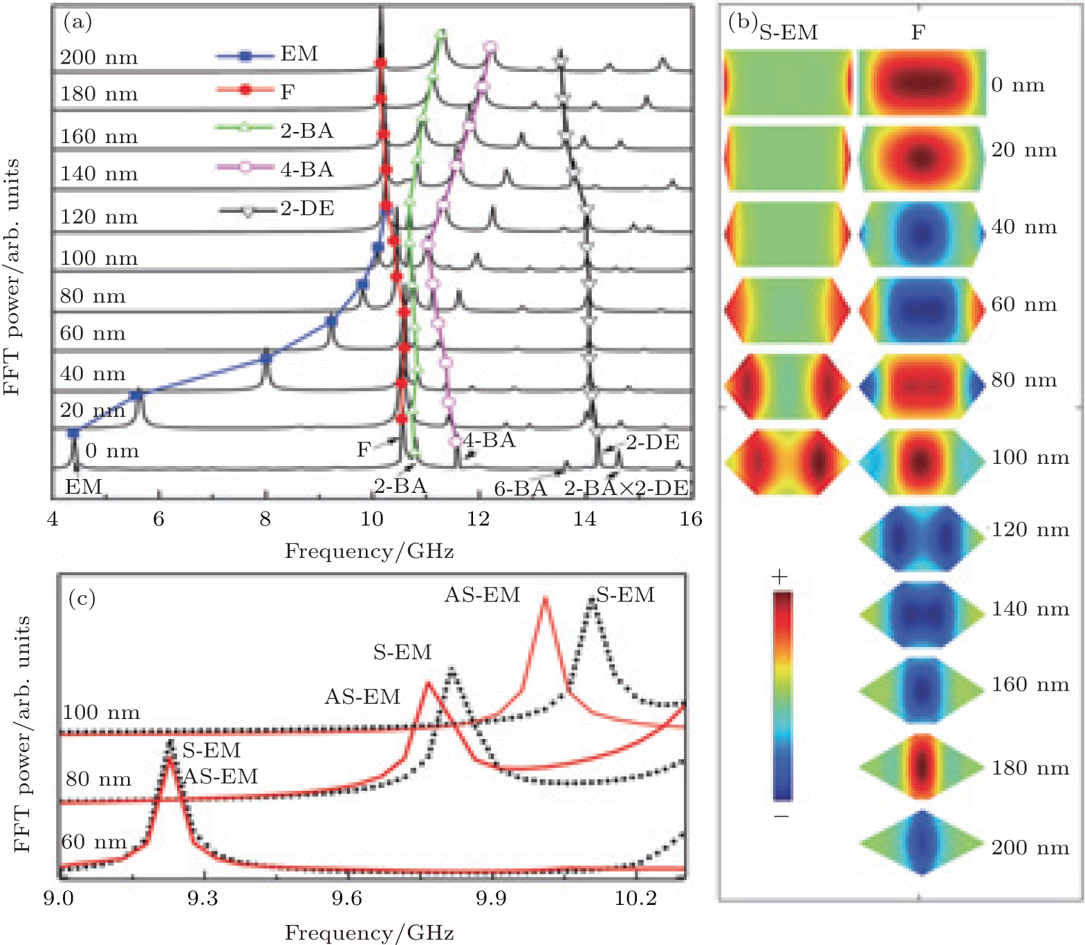Fig. 3. (a) Spin-wave resonance spectra of the elements with different h. The blue circular, red pentagram, green diamond-shaped, magenta square, and black triangle dots denote the EM, F, 2-BA, 4-BA, and 2-DE modes, responsively. (b) Spatial profiles of the z-component of the dynamical magnetization of EM and F modes for different h. (c) Frequency evolution with h for degenerate S-EM and AS-EM modes.

The localization of the spin wave is strongly dependent on the distribution of the internal magnetic field. As for the edge mode, it is localized at the ends of the element where the internal magnetic field is strongly inhomogeneous, as shown in Fig. 4, where the simulated distribution of the internal field in elements with different h is depicted. The edge mode can exist only in a limited range of the internal field H_int (H_min(x) < H_int(x) < H_max(x)). It can be seen from Fig. 4 that, with the increase of h (but less than 100 nm), the inhomogeneous area of the internal field increases and expands toward the central area of the elements, which means that the field gradient along the x direction decreases with the increase of h. The change pattern of the internal field with h indicates the change form of the edge mode, i.e., the expansion and movement toward the central part of the element. Moreover, with the movement of the edge mode toward the centre, the internal field in the mode-localized area increases, which gives rise to the increase of the mode frequency. However, when h> 100 nm, the inhomogeneity of the internal field becomes sharp again and is even sharper than that of the inhomogeneity of the internal field in the rectangle element. In this case, the edge mode cannot be confined in such narrow area and it then disappears.

Fig. 4.

	Figure Option ViewDownloadNew Window
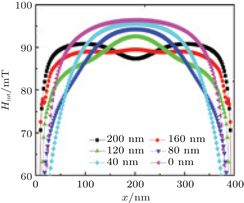	Fig. 4. Variation of the simulated internal field Hint along the element central line in the x direction.

To better understand how the spin-wave modes can be manipulated by changing the element shape, we carried out an analytical study based on an approximated spin wave dispersion relation for a uniformly magnetized rectangular element, ^[37] which can be described by

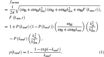
Here, ω _H = γ H_int describes the internal field contribution. The term is the dynamic exchange contribution, where ω _M = γ M_s and a = 2A_ex/(μ ₀M_s), F(k_mn, t) describes the dynamic dipole– dipole interaction, and t is the thickness of the element. The two-dimensional quantization wave vector is = k_me_x + k_ne_y, and The dispersion relation (1) has been applied to describe spin-wave modes in samples of different geometries and dimensions from thin films to isolated nanomagnets, such as elliptical nanodots^[16] and triangular nanodots, ^[11] and the results based on the formula are in agreement with the simulations, and are even in agreement with the experimental data. For numerical calculation of the frequency from Eq. (1), a key point is to determine the quantized wave numbers k_m and k_n. The wave number k_m can be approximated by k_m = (m + 1)π /Δ l_m, where Δ l_m is the effective localization length for a given spin-wave mode, which can be estimated approximately by the spatial image of the mode following the methods in Ref. [36]. As for k_n, taking the dipolar pinning boundary condition into account, it can be written as k_n = nπ /w_n. The w_n is supposed to be wd(p)/(d(p) − 2), ^[38] where d(p) = 2π /p[1 + 2ln(1/p)] is the effective pinning parameter, p = t/w, t = 5 nm is the thickness, and w is the width of the element. Taking the estimated k_m and k_n values and the internal field H_int obtained from the micromagnetic simulation results, the spin-wave mode frequencies can be calculated from Eq. (1). As H_int is inhomogeneous, especially in the end areas of the elements, it is taken to be the average internal field in the spin-wave localized area. Figure 5 shows the calculated dependence of the frequencies for different spin-wave modes on the tapered parameter h, together with the simulated results. It can be seen that the frequencies calculated from Eq. (1) are in reasonable agreement with the simulated results.

Fig. 5.

	Figure Option ViewDownloadNew Window
	Fig. 5. Dependence of the mode frequencies on taper parameter h. The solid and open dots denote the simulated and calculated data, respectively.

In summary, we have investigated the magnetization dynamics of nanoelements with tapered ends by using micromagnetic simulations. It is found that the dynamical properties can be tuned by changing the sharpness of the element ends. The edge mode is the most tunable spin-wave mode, which is localized in the two ends of the element. There is a critical tapered parameter h₀ (≈ 100 nm) below which the edge mode frequency increases rapidly with h and its localized area gradually expands toward the element center and finally merges into the fundamental mode at h₀. The degeneracy of the in-phase (S-EM) and out-of-phase (AS-EM) edge modes are gradually lifted with the increase of h. For elements with h > 100 nm, the edge mode disappears. Other spin-wave modes are less affected by tapering the element ends. The shifts of the frequencies for these modes are small and display different tendencies. For F and 2-DE modes, the frequency decreases slightly with the increase of h. However, for 2-BA and 4-BA modes, the frequency decreases at first and then increases with the increase of h. The evolution of the spin-wave modes with the tapered parameter h is mainly determined by the internal field. The mode frequencies are calculated based on an analytical formula and agree approximately with the simulation results. The results obtained in this work provide a way to manipulate the magnetization dynamics of nanomagnets and, further, to control the magnetization reversal as needed, which is important for designing high-density storage devices based on magnetic nanoelements.