


Landau level transitions in InAs/AlSb/GaSb quantum wells
[Wu Xiao-Guang†a)  , Pang Mi
b) ]
, Pang Mi|
|


†Corresponding author. E-mail: xgwu@red.semi.ac.cn
*Project supported by the National Natural Science Foundation of China (Grant Nos. 61076092 and 61290303).
The electronic structure of InAs/AlSb/GaSb quantum wells embedded in AlSb barriers and in the presence of a perpendicular magnetic field is studied theoretically within the 14-band k· p approach without making the axial approximation. At zero magnetic field, for a quantum well with a wide InAs layer and a wide GaSb layer, the energy of an electron-like subband can be lower than the energy of hole-like subbands. As the strength of the magnetic field increases, the Landau levels of this electron-like subband grow in energy and intersect the Landau levels of the hole-like subbands. The electron–hole hybridization leads to a series of anti-crossing splittings of the Landau levels. The magnetic field dependence of some dominant transitions is shown with their corresponding initial-states and final-states indicated. The dominant transitions at high fields can be roughly viewed as two spin-split Landau level transitions with many electron–hole hybridization-induced splittings. When the magnetic field is tilted, the electron-like Landau level transitions show additional anti-crossing splittings due to the subband-Landau level coupling.
In recent decades, the transport and optical properties of InAs/GaSb quantum wells have been investigated experimentally and many interesting features have been revealed.[1– 13] Among various experimental techniques, the Landau level spectroscopy has been employed in exploring the electronic properties of InAs/GaSb quantum wells. A key element in understanding those experiments is the electron– hole hybridization.[14] At low magnetic fields, the agreement between the experiments and theories seems to be fairly good.[15] However, at high magnetic fields, the difference between the experimental data and the theoretical simulation is small for some quantum structures, but is not small for some other structures.[10] A dominant transition is observed at high magnetic fields, but this is unexpected as the corresponding initial state should be empty.[10] In a more recent experimental study, without a direct comparison to a theoretical simulation, it was pointed out that the conventional model cannot account for the observed features, and one needs to introduce a spontaneous phase separation for the nominally uniform InAs/AlSb/GaSb quantum wells.[11]
Most previous theoretical works on the Landau level transitions in InAs/AlSb/GaSb quantum wells are based on the six-band or eight-band k · p approach.[15– 17] Usually, the transition energy is given but the transition strength is not shown. Furthermore, the axial approximation is often used in these theoretical calculations. When the axial approximation is employed, some couplings between Landau levels are ignored, and the influence of bulk inversion asymmetry, which is present in the system, is usually ignored. For HgTe quantum wells, where the electron– hole coupling is also important, it is necessary to avoid these approximations in order to understand some experimental results.[18– 20] Another potential problem is the possibility of spurious solution.[21, 22] It is known to occur in the calculation of electronic states in some InAs/GaSb superlattices within the eight-band k · p approach. Thus, it is better for one to go beyond the eight-band k · p method in the study of InAs/AlSb/GaSb quantum wells.
In the present paper, we investigate theoretically the electronic structure of InAs/AlSb/GaSb quantum wells embedded in AlSb barriers and in the presence of a perpendicular magnetic field within the 14-band k · p approach without making the axial approximation. The energies of some Landau level transitions and their corresponding transition strengths are calculated. The magnetic field dependence of some dominant transitions is displayed together with their corresponding initial-states and final-states indicated. This information should be useful in analyzing an experimentally measured magneto– optical spectrum. Unfortunately, a quantitative comparison with the experiments is not yet possible, as the distribution of donors and acceptors in the experimental samples is unknown. The knowledge of this distribution is necessary in determining the magnetic field dependence of the self-consistent potential. This self-consistent potential affects the relative position of the electron-like and the hole-like subbands and hence the features shown in the magnetic field dependence of the Landau level transitions. We hope that the present theoretical work will inspire more experimental investigations.
This paper is organized as follows: In Section 2, the theoretical formulation is briefly presented. Section 3 contains our calculated results and discussion. Finally, in the last section, a summary is provided.
The calculation of one-electron energy levels is based on the well documented k · p approach.[23] For details about this method, e.g., the operator ordering, the inclusion of a magnetic field, the influence of remote bands, the influence of strain, and the modification due to heterojunction interfaces, we refer to a partial list of publications and references therein.[24– 32] In our calculation, the influence of strain is included and is found to be important quantitatively. The quantum well is assumed to be parallel to the xy plane, and the external magnetic field is along the z direction. In our calculation, the axial approximation is not used as mentioned in the introduction. A plane wave and Landau level expansion scheme is used, and we have checked carefully that there is no spurious solution in our calculated electronic states. The material parameters used in the calculation can be found in the literature, [32, 33] and no other adjustable parameter is introduced.
After obtaining the electronic energy levels, transition energies can be easily calculated. In order to know the nature of a transition, we also calculate the corresponding optical transition matrix elements between two involved states.[34, 35] Assuming the two states are denoted as | 1〉 and | 2〉 , we will calculate π x = | 〈 1| (px + eAx/c)| 2〉 | 2, and π y = | 〈 1| (py + eAy/c)| 2〉 | 2. Because of the reduced symmetry in the InAs/GaSb quantum wells, two matrix elements π x and π y are not identical, but almost the same for the quantum wells studied in this paper. In the calculation of the above matrix elements, one should take into account the contribution from the Bloch basis states, as the inter-subband optical transition is not fundamentally different from the inter-band optical transition.
For simplicity, we will ignore the depolarization field correction[36– 38] due to the dynamic space charge effect in the quantum well. We believe that this is a reasonable approximation, when the magnetic field is not tilted, as the transitions involved have their initial-states and final-states from the same subband. The lack of detailed knowledge about the carrier distribution also makes the investigation of this many-body effect difficult. The exchange and excitonic effects due to the electron– electron interaction[39] will also be ignored for simplicity in the present work, and will be studied in the future.
The InAs/AlSb/GaSb quantum wells studied in the present paper have the following structure: the AlSb left-barrier, the InAs layer, the thin AlSb layer, the GaSb layer, and finally the AlSb right-barrier. The growth direction of the quantum wells is assumed to be [001]. The model quantum well includes a thin layer of AlSb between the InAs and GaSb layers. The inserted thin AlSb layer can control the degree of electron– hole hybridization.[10, 11] The width of InAs layer will be varied, so that the relative positions of the electron-like and the hole-like subbands can be changed. The width of inserted AlSb layer will also be varied. The width of GaSb layer will be fixed, so that the hole-like subbands are roughly unchanged in energy.
In Fig. 1, the magnetic field dependence of Landau levels is shown for two InAs/AlSb/GaSb quantum wells. In the upper panel, the width of InAs layer is 130 angstrom, and in the lower panel, the width of InAs layer is 170 angstrom. In both panels, the width of AlSb layer is 10 angstrom, and the width of GaSb layer is 50 angstrom. The quantum well structure information is explicitly shown in Fig. 1 as QW:130/10/50 in Fig. 1(a), and as QW:170/10/50 in Fig. 1(b). The top of conduction band of InAs is taken as the energy zero point.
 | Fig. 1. Magnetic field dependence of Landau levels of InAs/AlSb/GaSb quantum wells. In panel (a), the width of InAs layer is 130 angstrom, and in panel (b), it is 170 angstrom. The width of AlSb layer is 10 angstrom, and the width of GaSb layer is 50 angstrom. When the largest component of a state is from the conduction band, the dot symbol for the state energy is colored red for the spin-down state, and is colored green for the spin-up state. The top of the conduction band of InAs is taken as the energy zero point. The quantum well structure information is denoted as QW:130/10/50 in panel (a), and as QW:170/10/50 in panel (b). |
The wave functions of some states are calculated. By analyzing the wave function of a state, one can easily determine that the state is an electron-like (the conduction band contribution dominant) state or it is a hole-like (the valence band contribution dominant) state. One can also determine the Landau level index of its dominant contribution. In Fig. 1, when the largest component of a state is from the conduction band, the energy of the state is colored red for the spin-down state, and it is colored green for the spin-up state. From Fig. 1, one can roughly identify the fan shape of the Landau levels of those electron-like states. However, the spin-up and spin-down electron-like Landau levels can no longer form smooth fan-shape lines because of the electron– hole hybridization. One sees that usually a spin-up electron-like state has a lower energy than the corresponding spin-down electron-like state. This means that the g-factor is negative for the electron-like states similar to the case of bulk InAs and the case of InAs quantum wells.
In the energy window shown in Fig. 1, the states whose energies fall between the electron-like states are the hole-like states. As the width of GaSb layer is fixed, the position of hole-like states remains roughly unchanged, while the energies of electron-like states decrease as the width of InAs layer increases. This is expected, as the electron-like states are confined by the outer AlSb barriers. The slope of electron-like Landau levels also changes as the InAs layer width varies. This is due to the non-parabolic band effect.
We find that the top energy levels, at about 0.11 eV, of the hole-like subband are zero index Landau levels. At high magnetic fields, the zero Landau levels from the electron-like subband will grow in energy and intersect those hole-like zero Landau levels. There are small anti-crossing gaps but these cannot be seen with the energy scale in Fig. 1. This zero Landau level anti-crossing can be attributed to the influence of bulk inversion asymmetry.[18– 20]
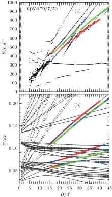
Next, let us examine the Landau level transitions. In Fig. 2, for the QW:130/10/50 quantum well (the width of InAs layer is 130 angstrom, the width of AlSb layer is 10 angstrom, and the width of GaSb layer is 50 angstrom), the energies of some Landau level transitions are shown in Fig. 2(a) as a function of the magnetic field strength. The energy levels versus the magnetic field are shown in Fig. 2(b) for the same quantum well structure.
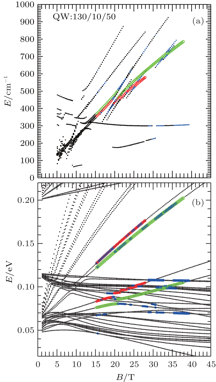 | Fig. 2. Panel (a) shows the energy of some Landau level transitions (open circles) versus the magnetic field for the QW:130/10/50 quantum well. The widths of InAs, AlSb, and GaSb layers are 130, 10, and 50 angstrom, respectively. Panel (b) shows the energy levels versus the magnetic field for the same quantum well structure. These transitions are from states with energy lower than 0.105 eV to states with energy higher than 0.105 eV. The size of the open circles in panel (a) is proportional to the corresponding transition strength π x. At a fixed magnetic field, the first three most dominant transitions according to the corresponding π x values are colored red, green, and blue. The corresponding initial-states and final-states of the Landau level transitions are indicated in panel (b) with the same color. The initial-states are marked as open circles, the final-states are marked as open squares or open diamonds. |
These transitions are from the states with energy lower than 0.105 eV to the states with energy higher than 0.105 eV. The selection for the Landau transitions is made because the transitions between the electron-like Landau levels must be included. These transitions are most relevant to a magneto-spectroscopy experiment.[11] Some transitions from low lying states to a few top hole-like Landau levels with low Landau level index are also included, as the experimental samples usually contain electrons as well as holes.[10, 11] In the present work, we will make the same selection for the Landau level transitions, thus one has a consistent view.
For a given magnetic field, the energy of a Landau level transition is plotted in Fig. 2(a) as an open circle. The size of the open circle is proportional to the corresponding transition strength π x. At a fixed magnetic field, the first three most dominant transitions according to their π x values are colored. It will be colored red if the corresponding initial-state is a spin-down electron-like state. It will be colored green if the initial-state is a spin-up electron-like state. If it cannot be colored red or green, it will be colored blue. In Fig. 2(b), the corresponding initial-state and final-state of the Landau level transition are indicated with the same color. The initial states are marked as open circles, the final states are marked as open squares or open diamonds. Different symbol sizes are used in Fig. 2(b) so that one can clearly see two transitions with the same final-states. We will focus on the high magnetic field region, B > 15 T, as our calculated results can be presented more clearly.
It must be pointed out that the strength of a mode observed in a magneto-spectroscopy experiment also depends on the involved sample carrier density. A transition will not be detected experimentally if the initial-state is empty or the final-state is fully occupied. We believe that the information in the way it is provided in Fig. 2 should be useful in analyzing an experimentally measured magneto– optical spectrum.
In Fig. 2, one sees that, at high magnetic fields, B > 15 T, the dominant Landau level transitions can be viewed roughly as two spin-split Landau level transitions with many electron– hole hybridization-induced splittings. Two large hybridization-induced splittings occur at the magnetic field around 20 T. For magnetic fields in the interval from 15 T to 20 T, the distance between two dominant transitions is almost field independent first, then decreases. When the magnetic field is higher than 20 T, the distance between two dominant transitions increases slightly as the magnetic field increases. From the lower panel of Fig. 2, one sees that, at high magnetic fields, the splittings in the Landau level transitions are due to the electron– hole hybridization-induced initial-state splittings.
In Fig. 2, one can observe electron– hole hybridization-induced multiple splittings on the dominant Landau level transition at a very high magnetic field about 34 T. This splitting occurs because the n = 1 hole-like Landau level has a non-monotonic magnetic field dependence. The n = 0 electron-like Landau level shows anti-crossings with this n = 1 hole-like Landau level at about 34 T. It is clear that the size of the splittings is much smaller than the splitting that occurred at the magnetic field about 20 T also due to the anti-crossing of the n = 0 electron-like Landau level and the n = 1 hole-like Landau level. In a magneto-spectroscopy experiment, this splitting in the high magnetic field may manifest as a resonance line-width broadening, if the splitting is not fully resolved.
The degree of electron– hole hybridization can be tuned by changing the width of the inserted AlSb layer. In Fig. 3, the Landau level transition energy versus the magnetic field strength is shown in Fig. 3(a) for the QW:130/5/50 quantum well. The AlSb layer width is reduced to 5 angstrom and the electron– hole hybridization hence becomes stronger. Figure 3(b) shows the energy levels versus the magnetic field for the same quantum well structure. By comparing Figs. 2(b) and 3(b), one can clearly see the influence of this stronger electron– hole hybridization on the energy levels. At high magnetic fields, B > 15 T, the first 3 most dominant transitions are colored in the same way as that shown in Fig. 2. One sees that, at high magnetic fields, the magnetic field dependence of the Landau level transition energy shows a similar behavior as that displayed in Fig. 2. As one expected, the hybridization-induced splittings around 20 T become larger, thus the Landau level transitions also show larger splittings. For the magnetic fields between 15 T and 20 T, the distance between two dominant transitions also becomes larger. One can still roughly view the dominant transitions at high magnetic field, B > 15 T, as two spin-split Landau level transitions with many electron– hole hybridization induced splittings.
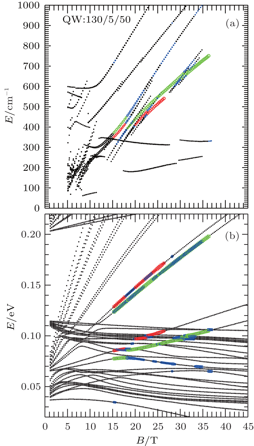 | Fig. 3. The same as Fig. 2, but for the QW:130/5/50 InAs/AlSb/GaSb quantum well. Panel (a) shows the energy of some Landau level transitions (open circles) versus the magnetic field. Panel (b) shows the energy levels versus the magnetic field. |
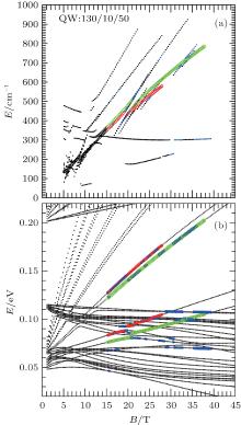
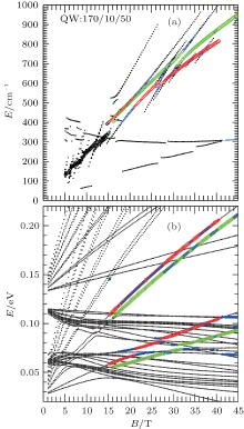
Next, let us examine InAs/AlSb/GaSb quantum wells with a wider InAs layer. When the width of the InAs layer increases, the energy of an electron-like subband decreases, the gap between two electron-like subbands becomes smaller. For the QW:130/10/50 quantum well, there is one hole-like subband between two electron-like subbands. For the QW:170/10/50 quantum well, there are two hole-like subbands between two electron-like subbands. The Landau level transition energies are shown versus the magnetic field in Fig. 4(a) for the QW:170/10/50 quantum well, and in Fig. 5(a), for the QW:170/7/50 quantum well. The widths of InAs and GaSb layers are the same, only the widths of inserted AlSb layers have a small difference. At high magnetic fields, B > 15 T, the transition energies are displayed and colored in the same way as that in Fig. 2. In Figs. 4(b) and 5(b), the energy levels are shown as a function of the magnetic field with the initial-states and final-states of Landau level transitions indicated.
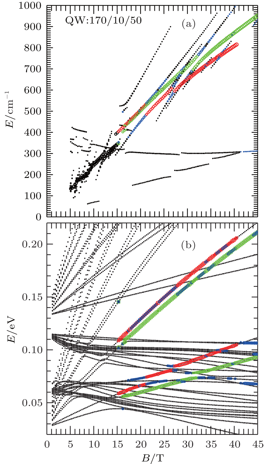 | Fig. 4. The same as Fig. 2, but for the QW:170/10/50 InAs/AlSb/GaSb quantum well. Panel (a) shows the energy of some Landau level transitions (open circles) versus the magnetic field. Panel (b) shows the energy levels versus the magnetic field. |
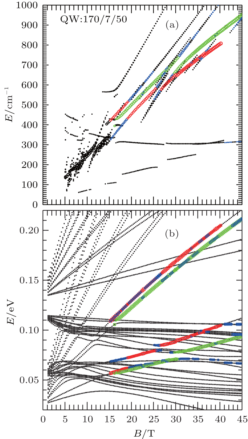 | Fig. 5. The same as Fig. 2, but for the QW:170/7/50 InAs/AlSb/GaSb quantum well. Panel (a) shows the energy of some Landau level transitions (open circles) versus the magnetic field. Panel (b) shows the energy levels versus the magnetic field. |
In Fig. 4, when the magnetic field falls between 15 T and 20 T, two dominant transitions almost coincide. When the width of inserted AlSb layer is reduced from 10 to 7 angstrom, one can see clearly in Fig. 5 that the distance between these two dominant transitions becomes larger. It should be pointed out that, one can still roughly view the dominant transitions at high magnetic fields, B > 15 T, as two spin-split Landau level transitions further split by many more electron– hole hybridization-induced splittings.
The tilting of the magnetic field is a technique often used in a magneto-spectroscopy experiment.[10, 11] One could obtain some information about the subband gap by tilting the field. In Fig. 6, the Landau level transition energies and energy levels are shown as a function of the total magnetic field strength for the QW:170/10/50 quantum well. The magnetic field is tilted 12.5 degree along the [100] direction. The transition energies and Landau levels are displayed and colored in the same way as that shown in Fig. 2. However, the first 4 dominant transitions are colored here. As expected, one sees that the tilted magnetic field induces a subband-Landau level anti-crossing at about 35 T. This anti-crossing field can be reduced when one increases the width of the InAs layer, thus reducing the energy gap between the electron-like subbands. By examining cases with different tilting angles, we find that the tilting of the magnetic field introduces mainly a subband-Landau level coupling with the same spin. One sees that this subband-Landau level coupling affects the final-states more strongly, and has a smaller effect on the initial-states. For the magnetic field lower than 30 T, the magnetic field dependence of Landau level transitions is not strongly modified. This can be clearly seen by comparing Fig. 6 with Fig. 4. This feature is also observed in a recent experiment.[11] It is interesting to note that the electron– hole hybridization-induced splittings can still be seen in the magnetic field region where the subband-Landau levels are strongly coupled. It should be pointed out that the depolarization correction may become important when the magnetic field is tilted. However, one needs the information about the carrier distribution in order to take this effect into account.
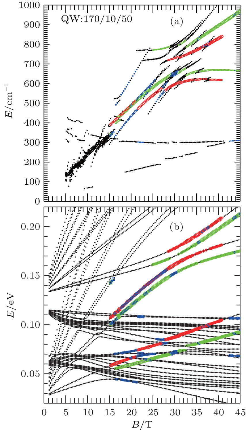 | Fig. 6. The same as Fig. 2, but for the QW:170/10/50 InAs/AlSb/GaSb quantum well. Panel (a) shows the energy of some Landau level transitions (open circles) versus the magnetic field. Panel (b) shows the energy levels versus the magnetic field. The magnetic field is tilted 12.5 degrees. The first 4 dominant transitions are colored. |
In summary, the electronic structure of InAs/AlSb/GaSb quantum wells embedded in AlSb barriers and in the presence of a perpendicular magnetic field is studied theoretically within the 14-band k · p approach without making the axial approximation. The energies of some Landau level transitions and their corresponding transition strengths are calculated. The magnetic field dependence of some dominant transitions is shown with their corresponding initial-states and final-states indicated. This information should be useful in analyzing experimentally measured magneto– optical spectra. We find that, at high magnetic fields, the dominant Landau level transitions can be roughly viewed as two spin-split Landau level transitions further split by many more electron– hole hybridization-induced splittings.
| 1 |
|
| 2 |
|
| 3 |
|
| 4 |
|
| 5 |
|
| 6 |
|
| 7 |
|
| 8 |
|
| 9 |
|
| 10 |
|
| 11 |
|
| 12 |
|
| 13 |
|
| 14 |
|
| 15 |
|
| 16 |
|
| 17 |
|
| 18 |
|
| 19 |
|
| 20 |
|
| 21 |
|
| 22 |
|
| 23 |
|
| 24 |
|
| 25 |
|
| 26 |
|
| 27 |
|
| 28 |
|
| 29 |
|
| 30 |
|
| 31 |
|
| 32 |
|
| 33 |
|
| 34 |
|
| 35 |
|
| 36 |
|
| 37 |
|
| 38 |
|
| 39 |
|