

Distribution characteristics of intensity and phase vortices of speckle fields produced by N-pinhole random screens
[Liu Man†a), b)  , Cheng Chuan-Fu‡
b) , Ren Xiao-Rongb) ]
, Cheng Chuan-Fu‡, Ren Xiao-Rong|
|


†Corresponding author. E-mail: lium7879@163.com
‡Corresponding author. E-mail: chengchuanfu@sdnu.edu.cn
*Project supported by the National Natural Science Foundation of China (Grant No. 11404179).
We analyze the distribution properties of phase and phase vortices in a speckle field generated by N-pinhole random screens, and find that the phase vortex distributions show similarity and clustering in local regions. The phase patterns have a lot of sets composed of two phase vortices with opposite signs or four phase vortices which are positive and negative vortices alternately. Cases are also found where two adjacent phase vortices have the same topological charges. The density of phase vortices becomes larger with the increase of the radius of circumference and the number of pinholes on screen. Then, the relative positions of phase vortices can be adjusted by changing the radius of circumference and the number of pinholes.
When coherent light waves are scattered from the random surfaces or the random media, speckles are formed in diffraction regions.[1] Usually, speckle patterns depend on the properties of the scatterer and the scattering aperture. When the scattering aperture is the multi-pinhole case, the speckle patterns differ from that generated by a single aperture. In the early studies, speckle photography with multi-aperture such as two-, three-, and four-pinholes has been studied, however, which is mainly used in the area of deformation and strain analysis. For example, Duffy[2] used a double aperture arrangement to record speckles for in-plane displacement. Chiang et al.[3] gave a detailed analysis of using multiple apertures to record laser speckles for strain analysis. In all these studies, the statistical properties of the speckles have rarely been involved.[4– 6] Recently, due to the cluster speckle having potential applications in optical manipulation, atoms trapping, speckle metrology, etc., the issue again has come into the views of researchers in the studies of speckle statistics.[7– 11] In speckle patterns, there are many dark points with vanishing intensity and undefined phase, and these points are so-called phase singularities or phase vortices.[12] Ten years ago, an accurate mapping between the intensity of the speckle field and the atomic density was found, the speckle fields were proposed to trap and cool atoms, [13, 14] when the tiny particles on the arbitrary phase vortex points, it can be trapped by an optical trapping system. The sizes of speckle grains produced by multi-pinhole are reduced several times compared to usual speckles, so it can trap multiple particles at the same time. The speckle phase vortices have become an important branch of optical vortices in recent years, [15, 16] and they have potential applications in many areas, such as geological structure and ice detection, medical examination, testing, and other areas of aerospace components.[17– 21] What is more important is that many experimental and theoretical studies have been performed on the nearest neighbor anti-correlations, statistical probability densities, and local properties of the phase vortices in a speckle.[22– 24] Since the speckle patterns differ in a cluster produced by multi-pinhole random screens, the phase distributions and the characteristics of phase vortices may be different from those generated by single aperture. To the best of our knowledge, the statistical characteristics of phase distributions and the phase vortices in cluster speckles have not been extensively studied. Therefore, it would be interesting to explore the characteristics of speckle phase vortices and their distributions produced by multi-pinhole aperture.
In this paper, we use the method of numerical simulation to analyze the phase vortex distributions and phase patterns of speckle fields in the Fraunhofer diffraction region. We find that the phase patterns of the speckles have substructures which are similar, and the substructures are determined by the number of circular apertures N and the radius R of the circumference along which the pinholes are distributed uniformly. There are three new characteristics of phase distributions. Firstly, the same color regions appear repeatedly, which leads to non-uniform distribution of phase. Secondly, there are many units consisting of two phase vortices with opposite topological charges or four phase vortices with positive and negative vortices alternately appearing. We define those units as “ phase vortex sets” , around which the phase changes slowly. Thirdly, there are many phase vortex points which are arranged almost in a regular way and they form the positive and negative phase vortex lattices. Besides, the adjacent two phase vortices have the same topological charges in the local regions of phase patterns, around which the phase distribution is similar to vortex beams with the topological charges ± 2. These interesting new properties are different from those generated by a single circular aperture. With multi-pinhole random screens, we discuss qualitatively the phase and phase vortex distributions in the speckle fields, and the more calculations demonstrate that the phase distribution is related with the number of pinhole N and the radius R of the circumference. We also discuss quantitatively the phase distribution, the local probability distribution for phase change per unit geometrical angle and the local probability distribution of the eccentricities.
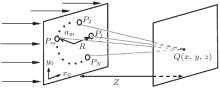
We consider the multi-pinhole random screen consisting of even-N small circular holes uniformly distributed along a circle with radius R in the x0y0 plane, as shown in Fig. 1. The radius of the pinholes is r, the azimuth angle of the m-th pinhole Pm is α m = 2π m/N(m = 0, 1, 2, … , N − 1), and z is the distance from the random screen to the observation plane. A parallel laser beam with wavelength λ and unity amplitude illuminates a refractive random screen in the x0y0 plane. The complex amplitude in the observation plane can be expressed as[25]

where h(x0, y0) is the surface height distribution, k = 2π /λ is the wave number, and n is the refractive index of the random screen. The aperture function T(x0, y0) of the random screen is written as

where (x0m, y0m) is the coordinate of the center of the m-th pinhole, and 
where A ≥ 0 is the amplitude, φ (x, y) is the phase with the range of (− π , π ], ξ (x, y) and η (x, y) are the real and the imaginary parts of the optical field, respectively. The intensity at point (x, y) is given by I = E(x, y)E(x, y)* . Generally, the phase change around a speckle phase vortex is not-uniform.[26] Close to a phase vortex, the contours of intensity are ellipses while the contours of current, J = | J| = I∇ φ , are circles. The current associated with E(x, y) current is defined as ω = ∇ × J/2 = ∇ ξ × ∇ η , the eccentricity ε of the intensity contours can be expressed as[26]
the variation of phase with geometric angle only depends on ε .[11] The more uniform the phase changes around a phase vortex, the smaller the eccentricity, and vice versa.
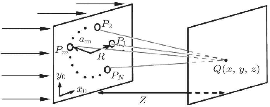 | Fig. 1. The geometry of multi-pinhole random screen and interference field. |
In the numerical calculation, we use the random numbers with the range of [− 1, + 1] to substitute the random screens for simplicity, the largest random number 1 represents the maximum surface height is 1.0 μ m. The values of z, λ , n, r, and R are set as 20.0 cm, 0.6328 μ m, 1.532, 4.0 μ m, and 42.0 μ m, respectively. The range of the observation plane is set as 6.0 × 6.0 cm2 with 1001 × 1001 sampling points.
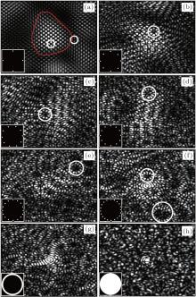
Based on Eqs. (1) and (2) and the above mentioned parameters, we calculate the speckle field produced by multi-pinhole random screens. The speckle intensity patterns generated by screens with hole numbers N = 4, N = 8, N = 10, N = 12, N = 16, and N = 20 are shown in Figs. 2(a)– 2(f), respectively. Figures 2(g) and 2(h) give the speckle intensity patterns produced by a large single ring aperture and by a large single circular aperture, respectively, for comparing the results in Figs. 2(a)– 2(f). The patterns in these figures are given in 32 gray scales with ranges from zero to the maximum intensity of each pattern. The inset in each pattern is the geometry of the apertures, the radii of a large single ring and circular aperture are the same as the radius of the circumference.
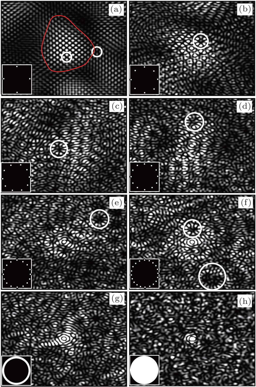 | Fig. 2. The intensity distribution patterns produced by the multi-pinhole, (a) N = 4, (b) N = 8, (c) N = 10, (d) N = 12, (e) N = 16, (f) N = 20, (g) a large single ring aperture and (h) a large single circular aperture, respectively. |
It can be seen that a bright large-sized speckle grain labeled by the red closed curve appears in the center of Fig. 2(a) for N = 4. Inside the large-sized speckle grain, there are small-sized speckle grains which are arranged in order and even distribution. In the dark regions of Fig. 2(a), there are also small-sized speckle grains, but their intensity is small and their distributions are out of order. The difference between the large bright and dark areas is particularly evident. Comparing Fig. 2(a) with Fig. 2(b), we find that the small-sized speckle grains in Fig. 2(a) are arranged regularly, the majority of which have a uniform size. However, the distributions of the small-sized speckle grains in Fig. 2(b) are irregular; they differ in size more obviously.
From Figs. 2(c)– 2(f), we can see that the borders of large-sized speckle grains become blurry with the increase of N, although large bright and dark areas still appear. In a certain region, the small-sized speckle grains are evolved into cluster structures, whose shapes and trends become more complicated with the increase of N. These cluster structures appear even in the ring aperture case. From Figs. 2(a)– 2(d), we can find that the small speckle grains with grain numbers of 4, 8, 10, and 12 respectively in the circled areas have a resembling distribution to those of the pinholes of the corresponding screens, and such a characteristic is more obvious for speckles of the smaller number screens in Figs. 2(a) and 2(b). We find that in Figs. 2(e) and 2(f) when pinhole numbers are equal to or greater than 16, the small-sized speckle grains are also arranged in cluster structures, but the number in the circled areas is not equal to the pinholes in the aperture, and the size of cluster structures is different. In the case of the large single ring aperture, the distribution of small-sized speckle grains in Fig. 2(g) is similar to that in Fig. 2(f) for a large single circular aperture, and they are arranged in different sizes of the circle or ellipse clustering. On the whole, with the increase of the pinhole numbers, the distributions of the small-sized speckle grains produced by multi-pinhole are more and more similar to those produced by the large single ring aperture. We believe that the small-sized speckle grains result from the complex modulation generated inside each speckle field, which is produced by multiple interferences of the different components of the angular spectrum of the random light waves. Due to the area of the autocorrelation function of speckle intensity in the Fraunhofer diffraction region doubling that of the aperture, [22] the tolerance of the distance between the adjacent pinholes is twice as large as the aperture radius r. Based on the screen geometry parameters in this paper, we can obtain that the optimized number of multi-pinholes is 10. The tolerance of the optimized screen geometry parameters can be adjusted according to the particle size.
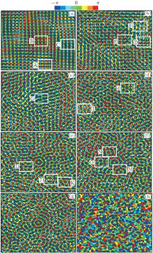
Next, we mainly focus on the characteristics of phase and phase vortex distributions in the Fraunhofer diffraction region. Figures 3(a)– 3(h) show color phase patterns in correspondence with the intensity patterns in Figs. 2(a)– 2(h), respectively. In Fig. 3, the dimensions of each pattern are 6.0 × 6.0 cm2 with the phases from – π to π represented by the color bars, and the black lines are equipages lines with phase increment of π /4. Some of the special phase distribution regions are labeled by white rectangles.
 | Fig. 3. The phase distribution patterns produced by the multi-pinhole aperture, (a) N = 4, (b) N = 8, (c) N = 10, (d) N = 12, (e) N = 16, (f) N = 20, (g) a large single ring aperture and (h) a large single circular aperture, corresponding to the patterns in Figs. 2(a)– 2(h), respectively. |
By comparing the phase patterns in Figs. 3(a)– 3(f) for the multi-pinhole cases with that in Fig. 3(h) for the large single circular aperture case, we may find that the phase patterns produced by the multi-pinhole random screens are obviously different from those by the single circular aperture. Figures 3(a)– 3(f) show that the distributions of the different color regions are clearly ununiform, the number of the phase vortices is larger than those in Fig. 3(h) and the phase vortex distributions appear to be similar and cluster in the local regions, such as the regions labeled by A, B, M, and N. However, in Fig. 3(h), we can find that all the colors distribute randomly on the whole pattern with each color taking almost a uniform proportion, the number of phase vortices is smaller than that for the multi-pinhole cases, and the phase vortex distributions are random.
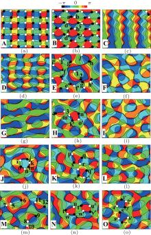
In order to observe more clearly the phase and phase vortex distributions in Figs. 3(a)– 3(g), we enlarge the regions labeled by the white rectangular boxes as A, B, C, D, E, F, G, H, I, G, K, L, M, N, and O, and they are shown in Figs. 4(a)– 4(o), respectively, where the dimensions of each pattern are 1.0 × 1.0 cm2 and the black-filled circles correspond to positive phase vortices and white-filled circles to negative phase vortices.
 | Fig. 4. Different local phase distribution patterns produced by the multi-pinhole aperture, with panels (a)– (o) corresponding to the enlarged regions A– O in Fig. 3. |
Figures 4(a)– 4(c) are in correspondence with the regions labeled by A, B, and C in Fig. 3(a) for the four-pinhole, respectively. We can see that the positive and negative phase vortex points shown in Fig. 4(a) are arranged almost in a regular way, and they form the positive and negative phase vortex lattices, of which the positive and negative phase vortices appear alternately. The phase around each adjacent positive and negative phase vortex is nearly symmetrically distributed. One positive (negative) phase vortex and its neighboring four negative (positive) phase vortices in the horizontal and vertical directions connect with two equiphase lines which have almost equal intervals. The shapes of the equiphase region are irregular quadrangles except for ellipse-like equiphase regions which distribute between two adjacent phase vortices having opposite signs. From Fig. 4(b), we can see that the probability for a phase to take the values around – π /2 or π /2 is small, and the sizes and the shapes of the same color regions are nearly equal. The positive and negative phase vortex points are still arranged regularly. The phase distributions around the adjacent positive and negative phase vortices are similar to each other, e.g., the phase vortex points labeled by letters a and b. The same color regions appear repeatedly, such as the red region is shared by four phase vortices labeled by letters a, b, c, and d, and the other region is shared by four phase vortices labeled by letters a′ , b′ , c′ , and d′ . One positive phase vortex and its neighboring negative phase vortex are connected with one to three equiphase lines whose lengths are different. In Fig. 4(c), the sizes of the different color regions are slightly different. The distributions of the same color regions appear as a striped structure whose phase values are repeated after the phase difference change 2π from left to right. A few phase vortices appear in this region.
Figures 4(d)– 4(f) correspond with the regions labeled by D, E, and F in Fig. 3(b) for an eight-pinhole, respectively. Comparing Fig. 4(d) with Figs. 4(a) and 4(b), we can still find that the shapes of the same color regions are irregular quadrangles, but the sizes are different. It is interesting to note that in the central area of Fig. 4(e) there is a positive– negative phase vortex pair marked with numerals 1 and 2, which is completely surrounded by the blue phase region and forms an independent unit. There are no equiphase lines connecting with other phase vortices, i.e., the eight equiphase lines radiate outward from one phase vortex point and then end on the other. Outside of the blue region, there are three positive– negative phase vortex pairs which share two to six equiphase regions, for instance, the vortex pairs labeled by letters i′ and f, j′ and g, l, and h, respectively. We can find that around the blue phase region, there are four phase vortices with the same topological charges marked by the letters e, f, g, and h, respectively, which are not connected with the blue phase region, there are also three phase vortices marked by the letters e′ , f′ , and g′ whose topological charges are alternately positive and negative, these three phase vortices connect with the blue phase region. Figure 4(f) shows that the sizes of the same color regions are different, and the probability for the phase to take the values around zero is small. Evidently, this demonstrates that the phase changes quickly around zero.
Figure 4(g) is the region labeled by G in Fig. 3(c) for a ten-pinhole, we note that the regions with the same color are elongated in the same direction. They form striped structures from top to bottom.
Figures 4(h) and 4(i) are the regions labeled by H and I in Fig. 3(d) for a twelve-pinhole. In Fig. 4(h), there is a phase vortex pair which is marked with numerals 3 and 4. This phase vortex pair shares six equiphase lines, and the remaining two equiphase lines end on the other phase vortex points, respectively. In the center of Fig. 4(h), there is a four-vortex set marked with m′ , n′ , o′ , and k′ , which contains two positive phase vortices and two negative phase vortices in an approximately symmetrical geometry. The phase of the red region surrounded by these four phase vortices varies slowly, but that between the adjacent phase vortices changes quickly, and outside of those four phase vortices the phase also changes slowly. The phase distributions in Fig. 4(i) are evidently nonuniform, which are similar to that in Fig. 4(f).
Figures 4(j)– 4(l) correspond with the regions labeled by J, K, and L in Fig. 3(e) for sixteen-pinhole, respectively. In Fig. 4(j), there is a six-vortex set marked with the letters i, j, k, m, n, and o, whose topological charges are alternately positive and negative. The phase surrounded by these six phase vortices changes slowly, but the phase between the adjacent phase vortices changes quickly, and the phase outside of those six phase vortices changes alternately in the range of [0, π ]. In Fig. 4(k), there are two four-vortex sets, which are marked with the letters p, q, r, and s, and p′ , q′ , r′ , and s′ , respectively. The phase distributions around the vortex points p and p′ are very similar, and the phase distributions around the vortex points q and q′ , r and r′ , s and s′ are also similar, moreover, the phase changes outside each four-vortex set are also similar. We define this phenomenon as “ local similarity” . In Fig. 4(l), we can see that the phase distributions of phase vortices are not regular, and the shapes of the regions of different colors are mostly irregular quadrangles.
Figures 4(m)– 4(o) correspond with the regions labeled by M, N, and O in Fig. 3(f) for a twenty-pinhole, respectively. It is not difficult to find from Fig. 4(m) that there are three positive-negative phase vortex sets which are marked with numerals 5 and 6, 8 and 9, 11 and 12, respectively. They share six to eight equiphase regions, and the size of equiphase region surrounding each the phase vortex pair is larger than the others, indicating that whose phases change relatively slowly. In Figs. 4(n) and 4(o), there are also two four-vortex sets, respectively, which are marked with the letters t, u, v and w, t′ , u′ , v′ and w′ in Fig. 4(n), and the numerals 1′ , 2′ , 3′ and 4′ , 5′ , 6′ , 7′ and 8′ in Fig. 4(o) respectively. Their distributions are similar to those in Fig. 4(k).
In addition to the above phenomena, we also find that some of the adjacent phase vortices have the same topological charge, which are like segregated second-order phase vortices, e.g., the phase vortices marked by the 2 and g′ in Fig. 4(e), 5 and 7, 8 and 10 in Fig. 4(m), respectively.
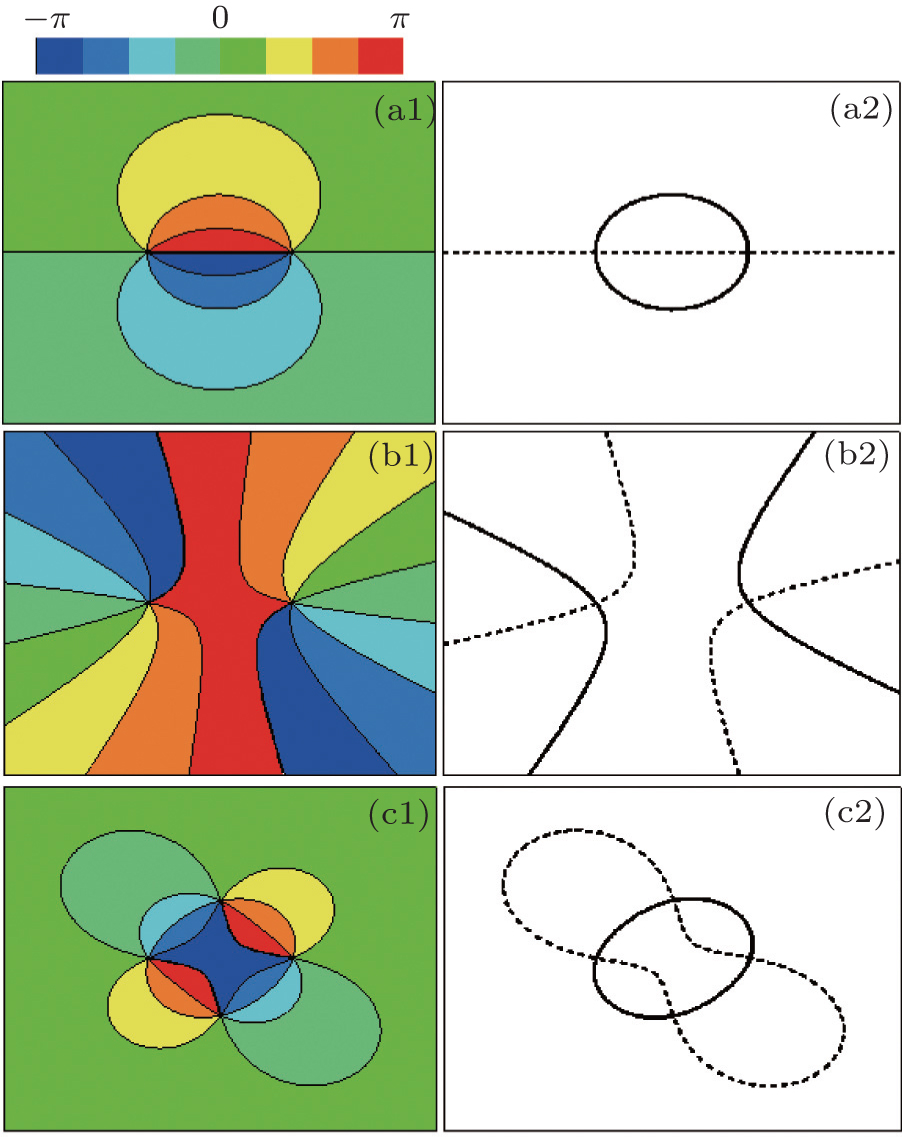 | Fig. 5. Distributions of phase and zero-crossings map of the real parts and the imaginary parts. (a) A pair of positive– negative phase vortices, (b) two positive phase vortices, (c) two pairs of positive– negative phase vortices, panels (a1), (b1), and (c1) are the zero lines of the real and the imaginary parts corresponding to panels (a), (b), and (c), respectively. |
On the whole, in Fig. 4, we may find that with the increase of the pinhole number, the numbers of the regions with positive and negative phase vortex lattices decrease, and the local similarity of phase distributions increases.
In order to explain qualitatively the phase vortex sets in the speckle fields produced by multi-pinhole in the Fraunhofer diffraction region, we use the method given by Freund[27] to simulate the phase vortices, as shown in Figs. 5(a1)– 5(c1). Figures 5(a2)– 5(c2) show the zero-crossing map of the real parts (black solid lines) and the imaginary parts (dashed lines) corresponding to Figs. 5(a1)– 5(c1).
Comparing the left column with the right column in Fig. 5, we find that when a zero line of the imaginary parts intersects with a closed zero line of the real parts, at the intersection they form a pair of positive– negative phase vortices; when two zero lines of the real parts and two zero lines of the imaginary parts intersect with each other respectively and around two intersections, the zero lines alternate the real parts and the imaginary parts, at these two intersections they form two phase vortices with the same signs; when a closed zero line of the real part intersects with a closed zero line of the imaginary part, four phase vortices appear at the intersections, forming a four-vortex set with the positive and the negative phase vortices appearing alternately.
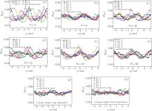
We next perform the quantitative analysis of the local similarity of the phase distribution produced with multi-pinhole random screens. We use data of phase patterns which are the same as in Fig. 4 for the statistical calculation. For each aperture, the data of the five different phase patterns are used for the statistics of the phase. Correspondingly, the five different random screens are labeled as No. 1, No. 2, No. 3, No. 4, and No. 5. The statistical results for all the cases are shown in Figs. 6(a)– 6(f), we define those curves as “ the local phase probability density distribution curves” , where the black solid lines are theoretical results based on the equation of[1]

From Figs. 6(a)– 6(f), we can see that the phase distributions of the speckle field produced by multi-pinholes random screens are nonuniform. The phase distributions produced by the five different random screens for the same aperture fluctuate in different degrees in each pattern. The probability for the phase to take the values around zero is larger in Figs. 6(b), 6(d)– 6(f), respectively. However, the local phase probability density distribution curves in Figs. 6(g) and 6(h) are roughly flat though some smaller fluctuations exist. In other words, the local phase distributions of the speckle field produced by both a large single ring aperture and a large single circular aperture are relatively uniform.
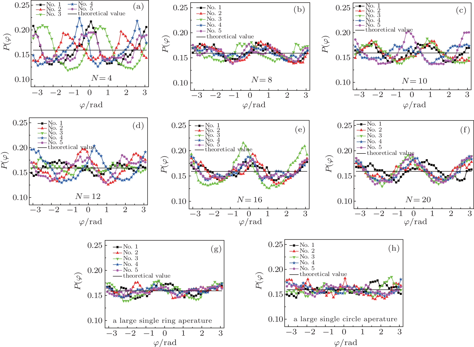 | Fig. 6. The local phase probability density distributions (a) N = 4, (b) N = 8, (c) N = 10, (d) N = 12, (e) N = 16, (f) N = 20, (g) a large single ring aperture and (h) a large single circular aperture. The solid lines are theoretical calculations. |
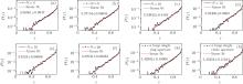
In the following, we analyze quantitatively the relation between the phase distributions and the eccentricities of the intensity contours around phase vortices. We first take each phase vortex point as the origin, then choose the length of 0.3 mm as the radius of a circle, on which we uniformly take 20 phase values and arrange these values in order starting from the minimum phase value, at the same time, record each phase value corresponding to each geometric angle θ (here, we introduce the partial derivative ∂ φ /∂ θ to represent the phase varies around the phase vortices), finally we obtain the local probability distribution P(∂ φ /∂ θ ) of ∂ φ /∂ θ . Our calculations of the local probability distributions P(∂ φ /∂ θ ) of the partial derivative for over 106 points for each case are shown in Fig. 7. By fitting the local P(∂ φ /∂ θ ) curves of ∂ φ /∂ θ in Cartesian coordinate, we obtain the slopes of all curves, and the results are shown in each pattern. From Fig. 7, we can see that when the values of ∂ φ /∂ θ are close to 0, the probabilities P(∂ φ /∂ θ ) reach a maximum value, and next the curves appear as a small fluctuation. In the range of 0.3 < ∂ φ /∂ θ < 2, the probability distribution curves fall much more rapidly, and then fall slowly for ∂ φ /∂ θ > 2. The data in each pattern increases with the increase of the pinhole numbers. When the pinhole number is equal to 12, the slope of the distribution curve reaches a maximum and then decreases.
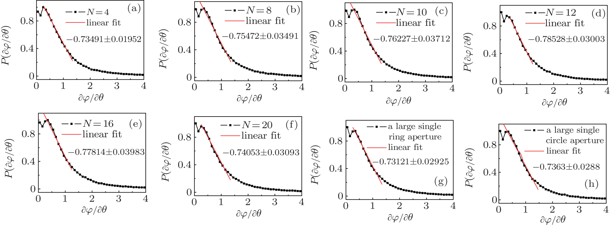 | Fig. 7. The local probability distributions of ∂ φ /∂ θ . (a) N = 4, (b) N = 8, (c) N = 10, (d) N = 12, (e) N = 16, (f) N = 20, (g) a large single ring aperture and (h) a large single circular aperture. |
Based on Eq. (4), we calculate the probability distribution P(ε ) of ε for over 104 phase vortices for each aperture. The results for all the cases are shown in Fig. 8. By fitting the probability distribution curves of the eccentricity in the logarithmic coordinate for all the cases, we obtain the slopes of all curves, and the results are shown in each pattern. We find that the slopes decrease with the increase of the pinhole numbers. When the aperture is 12-pinhole, the slope of the distribution curve reaches a minimum and then increases.
 | Fig. 8. The local probability distributions of ε . (a) N = 4, (b) N = 8, (c) N = 10, (d) N = 12, (e) N = 16, (f) N = 20, (g) a large single ring aperture and (h) a large single circular aperture. |
By comparing the data in Figs. 7 and 8, we may find that the number of phase vortices with a uniform phase distribution increase with the increase of the pinhole numbers, when the pinhole numbers are equals to 12, the number of phase vortices with uniform phase distribution reaches a maximum and then drops down.
The experimental measurement of the distribution of intensity and phase of speckle fields produced by N-pinhole random screens is not difficult to achieve. We can detect the intensity and phase with an experimental proposal as used in Ref. [16], only add a mask with multi-pinhole apertures immediately behind the random screen. Imaging methods were used to measure the intensity and interference pattern of speckle field, respectively. Then, the phase can be extracted from the interference intensity.
In summary, we analyze the distributions of phase vortices and phase in speckle field produced by multi-pinhole random screens, and find that the density of phase vortices becomes larger with the increase of the pinhole radius and the number of pinholes on aperture. In the local region of phase patterns, the phase vortex cluster phenomena, 2-order phase vortices and independent units composed by two phase vortices with opposite signs appear. We also obtain the corresponding relation between the probability distribution of slopes of the phase near the phase vortices and the eccentricities. These new phenomena have important significance in the studies of the essential structures, the new characteristics and new laws of phase vortices in speckle fields. Besides, our studies might also be used in optical trapping.
| 1 |
|
| 2 |
|
| 3 |
|
| 4 |
|
| 5 |
|
| 6 |
|
| 7 |
|
| 8 |
|
| 9 |
|
| 10 |
|
| 11 |
|
| 12 |
|
| 13 |
|
| 14 |
|
| 15 |
|
| 16 |
|
| 17 |
|
| 18 |
|
| 19 |
|
| 20 |
|
| 21 |
|
| 22 |
|
| 23 |
|
| 24 |
|
| 25 |
|
| 26 |
|
| 27 |
|