Multi-agent systems have attracted much attention in recent years. They offer many advantages over single agent systems, such as efficiency, robustness, scalability, versatility, adaptability, and lower cost.^[1] A considerable amount of research effort has been devoted to the distributed control of multi-agent systems. Examples of interesting research directions include consensus, ^{[2– 4]} formation control, ^{[5– 7]} coordinated tracking, ^{[8, 9]} flocking, ^{[10, 11]} and so on.

In the formation control problem, the agents are required to form a pre-defined formation shape, and then maintain the shape during translational or rotation movements. Rigid formation can keep the distance between any agent pair (the shape of the whole group) unchanged, which is not guaranteed by an arbitrary formation. Another feature of rigid formation is that it can be used to stabilize the distances between all of the agent pairs while employing the information of only a few agent pairs. This feature is of great significance in a large group of agents. Rigid formation control has found applications in various fields, including a wireless sensor network, surveillance, industrial processes, and so on.^{[1, 12, 13]} The objective of rigid formation tracking is to stabilize the relative positions of the agents according to a target rigid formation, while the agents can at the same time track a desired velocity. The incorporation of the desired velocity in formation control gives the system an extra ability to suit a complicated environment. However, this also complicates the design and analysis of the control algorithm. This paper is interested in the formation tracking problem for multi-agent systems via a rigidity framework.

The are many studies in the literature of formation control. In Ref.  [14], the global asymptotic stability of triangular formations is investigated. Local asymptotic stability of minimally infinitesimally rigid formations is analyzed by means of Lyapunov-based stability analysis.^[15] In Ref.  [16], a distributed coordinated tracking problem for multiple networked Euler– Lagrange systems is solved under the constraint that the leader is a neighbor of only a subset of the followers. A distance-based formation maintenance controller is designed for cycle-free persistent formations under the condition that the velocity of the trajectory is sufficiently low.^[17] For multi-agent formation maintenance and target tracking, a control law is developed in Ref.  [7], where the desired translational velocity and the leader’ s relative position and velocity are required by all of the followers. Using the relative positions of all of the agents, distance-based formation maintenance and target tracking schemes are solved by a modified gradient-of-potential-function law.^[18] Reference  [19] presents the design of control protocols and distributed observers for the leader-following formation control, which also deals with the formation as well as the tracking problem. In Ref.  [20], the consensus problem with a periodic intermittent communication and fixed directed topology is investigated, and then the consensus algorithm is extended to solve the formation control problem as well as the consensus tracking problem with switching directed topologies. Graph theory is a natural tool to describe multi-agent formation, a detailed discussion on the rigid graph theory and its applications is given in Ref.  [1].

The contributions of this paper are stated as follows. First, a desired group velocity is incorporated into the rigid formation control problem. When the desired velocity is time-varying, a distributed nonsmooth estimator is constructed to estimate the velocity and a Lyapunov function is provided to show the finite-time convergence of the estimator. Second, a formation acquisition term is derived from the rigidity matrix, which is used to solve the rigid formation control problem with the aid of the velocity estimator. Theoretical proofs are provided to show the convergence of the proposed formation control algorithms.

The rest of this paper is organized as follows. In Section  2, notation and mathematical preliminaries are presented. The formation control problem is defined in Section  3. Control algorithm design and stability analysis are presented in Sections 4 and 5, respectively, for the case of constant desired velocity and the case of time-varying desired velocity. Simulation results are given in Section  6. Finally, Section  7 summarizes the investigation.

Some basic knowledge on graph theory will be given in this section. An undirected graph is defined as , where is a set of vertices and is a set of undirected edges. The order and size of are denoted, respectively, by and . Denote the set of neighbors of vertex i by

Let p_i ∈ ℝ ² be the position of vertex i. A formation can be denoted by a pair (, p) where . Based on an arbitrary ordering of the edges in ℰ , an edge function : ℝ ²ⁿ→ ℝ ^m associated with (, p) is defined as

where ‖ · ‖ denotes the Euclidean norm. The rigidity of a formation is defined as follows.

Definition 1^[6] A formation (, p) is rigid if there exists a neighborhood of p ∈ ℝ ²ⁿ such that where Φ ^{− 1} is the set of the positions q ∈ ℝ ²ⁿ satisfying and is a complete graph of n vertices.

For a rigid formation, the distance between any two vertices will not change if the distances of the vertices corresponding to the edges which belong to the rigid graph remain unchanged during translation and rotation movements. The rigidity matrix R of a formation is given by

Obviously, the rigidity matrix only depends on the relative positions of the agents. Thus, we write the rigidity matrix as R(p̃ ) in the following, where p̃ _ij = p_i − p_j, (i, j) ∈ ℰ . Based on the rank property of R (p̃ ), the infinitesimal rigidity of F is defined as follows.

Definition 2^[6] A formation F = (, p), p ∈ ℝ ²ⁿ and n ≥ 3, is infinitesimally rigid in a two-dimensional space if rank[R(p̃ )] = 2n − 3.

Typically, formations that are rigid but fail to be infinitesimally rigid have collinear or parallel edges. In the following, the minimal rigidity of a formation is introduced.

Definition 3^[1] A formation is minimally rigid if it is rigid and no single interagent distance constraint can be removed without causing the formation to lose rigidity.

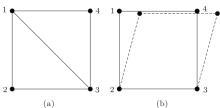
It can be verified that the graph in Fig.  1(a) is rigid. However, if any edge is removed from the graph, the graph is no longer rigid (see Fig.  1(b)). Thus, the graph in Fig.  1(a) satisfies Definition  3, and is said to be minimally rigid. In a two-dimensional space, a graph is minimally rigid if and only if m = 2n − 3.^[1]

Fig.  1.

	Figure Option ViewDownloadNew Window
	Fig.  1. Illustration of minimal rigidity.

Lemma 1 If a real matrix A ∈ ℝ ^{m× n} has full row rank, then AA^T is positive definite.

Proof For any x ∈ ℝ ^m, it follows that x^T(AA^T)x = (A^Tx)^T(A^Tx) ≥ 0. In particular, if x^T (AA^T)x = 0, then A^Tx = 0. Because A has a full-row rank, the equation A^Tx = 0 has one and only one solution x = 0. That is, x^T(AA^T)x = 0 has one and only has one solution x = 0, which suggests that AA^T is positive definite.

Consider a system of n agents governed by the single integrator dynamics

where is the position and u_i ∈ ℝ ² is the control input to be designed. Consider an infinitesimally and minimally rigid formation in ℝ ² described by , where and . Let F* be the desired formation, and denote the actual formation of the agents, where .

The objective of this paper is to design distributed controls u_i based on local information such that,

where υ _d (t) ∈ ℝ ² is any bounded, continuous function representing the desired velocity of the multi-agent system, and is available to only a subset of the agents.

In this section, we consider a case where the desired velocity v_d is constant. Define the relative position of two agents as

and let . The distance error is given by

The dynamics of the distance error are

Define the following positive definite, radially unbounded function:

The derivative of Eq.  (5) along Eq.  (4) is given by

From the definition of R(q̃ ), we know that each row of R(q̃ ) consists of q̃ _ij and q̃ _ji. Thus, Ẇ can be written in a vector form as

where and .

For each agent i, an estimator is designed to track the desired velocity v_d

where is the i-th agent’ s estimate of v_d, a_i0 > 0 if agent i has access to v_d, and a_i0 = 0 otherwise. We assume that there is at least one agent which has access to v_d.

The control input u is then designed as

where and k > 0. Let and . Note that v_d is constant. Equation  (7) can be written in a vector form as

where ℒ is the Laplacian matrix associated with , A₀ = diag(a₁₀, ..., a_n0), a_i0 ≥ 0 and there is at least one nonzero a_i0, and .

For a rigid graph, it is at least connected because otherwise if one or more nodes are not connected with other nodes, then this part of nodes can move freely without keeping distance to other nodes, which is in conflict with the nature of rigidity. Thus, is connected. It follows that H is positive definite.^[16] A Lyapunov function candidate V can be defined as follows:

where k is defined in Eq.  (8). Let . Define a level set Ω _c as

where c is a sufficiently small positive number.

The main result of this section is stated in the following theorem.

Theorem 1 For system  (1) under the control law  (8) and the estimator  (7), if F* is the desired formation and w(0) ∈ Ω (c), then the control objective  (2) and  (3) can be achieved, and the formation error and the estimation error converge to zero exponentially.

Proof The derivative of V along  (6) and  (9) is given by

Substituting Eq.  (8) into Eq.  (10) yields

Because , and it is straightforward to verify that σ ^T (e)R(q̃ )(1_n ⊗ v_d) = 0. It follows that

Because for w(0) ∈ Ω _c, we can conclude that w(t) ∈ Ω _c for all t ≥ 0. Because the target formation F* is infinitesimally and minimally rigid, R(q̃ * ) has a full row rank. From Lemma  1, we know that the matrix R(q̃ * )R^T(q̃ * ) is positive definite. The eigenvalues of R(q̃ * )R^T(q̃ * ) are continuous functions of the elements of the matrix. This is because the coefficients of the characteristic polynomial of a matrix is a continuous function of the elements of the matrix, and the eigenvalues of the matrix are continuous functions of the coefficients. Thus, for a sufficiently small positive number c, w ∈ Ω (c) can ensure that q̃ belongs to the open neighborhood where R(q̃ )R^T(q̃ ) has a positive minimal eigenvalue. Define the set S = {q̃ | λ _min[R(q̃ )R^T(q̃ )] > 0}, where λ _min denotes the minimum eigenvalue. It follows that

where inf(S) denotes the infimum of set S, and λ = min{2k inf(S), 1/λ _max[(H ⊗ I₂)^{− 1}]}. λ _max denotes the maximum eigenvalue. Thus, from Eq.  (11), it follows that σ (e) = 0, is exponentially stable.^[21]

The exponential stability of implies that ‖ q_i (t) − q_j (t)‖ → d_ij as t → ∞ for all (i, j) ∈ ℰ and as t → ∞ for all i ∈ . Finally, since σ (e) → 0 as t → ∞ and R(q̃ ) is bounded, we have that as Because we have proven that exponentially as t → ∞ , it follows from Eq.  (1) that q̇ _i (t) − v_d(t) → 0 as t → ∞ , i = 1, ..., n. The proof is thus completed.

In this section, we consider a case where v_d(t) is time-varying. It is assumed that the derivative of the desired velocity v_d(t) is bounded, and this bound is denoted by γ .

Inspired by Ref.  [8], the following non-smooth algorithm is proposed to estimate the time-varying desired translational velocity v_d(t):

where is the i-th agent’ s estimate of v_d(t), β is a positive constant, and sgn(· ) is the signum function. Define . The objective of  (12) is to guarantee that in finite time. The control law can be designed as

Theorem 2 For system  (1) under the control law  (13) and the estimator  (12), if F* is the desired formation, w(0) ∈ Ω (c), and β > γ , then the control objective  (2) and (3) can be achieved, and the formation error converges to zero asymptotically.

Proof In the following, we first prove that in finite time. From Eq.  (12), it follows that

Rewrite Eq.  (14) in a vector form as

where sgn(x) = [sgn(x₁), ..., sgn(x_n)]^T. Design the following Lyapunov function as:

The derivative of is given by

where represents the i-th element of . Recall that is bounded, and this bound is γ . It thus follows that

where It can be verified that there exists ɛ , such that

According to Theorem  3 in Ref.  [22], we can conclude that in finite time T, that is for i = 1, ..., n after time T.

After time T, the control law of (13) becomes

Substituting Eq.  (15) into Eq.  (6) yields

Following a similar proof to that of Theorem  1, it can be shown that R(q̃ )R^T(q̃ ) is positive definite for w(0) ∈ Ω _c. It thus follows that

The rest of the proof is similar to that of Theorem  1, and is hence omitted.

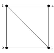
In this section, we present two simulation examples for the formation problem with constant and time-varying desired velocity, respectively. In both examples, we consider a group of four agents. The desired formation is a square shown in Fig.  2 where the agents are located at the four vertices. There are five edges in the graph. It can be verified that the formation given in Fig.  2 is minimally rigid. Let a₁₀ = 1, a₂₀ = a₃₀ = a₄₀ = 0. The desired distances between the agents are given by d₁₂ = d₂₃ = d₃₄ = d₄₁ = 10, The initial conditions of the agents are selected as and . The control gain k in Eqs.  (8) and (13) is set to 0.5, and β in Eq.  (12) is set to 1.2.

Fig.  2.

	Figure Option ViewDownloadNew Window
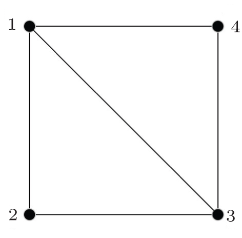	Fig.  2. Desired formation.

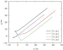
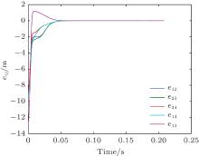
For the constant desired velocity case, let v_d = 1. Figure  3 shows the agents’ trajectories, which shows that the agents can achieve the formation asymptotically. Figure  4 shows that the inter-agent distance errors converge to zero. Figure  5 describes the velocities of all of the agents which converge to the desired velocity v_d = 1.

Fig.  3.

	Figure Option ViewDownloadNew Window
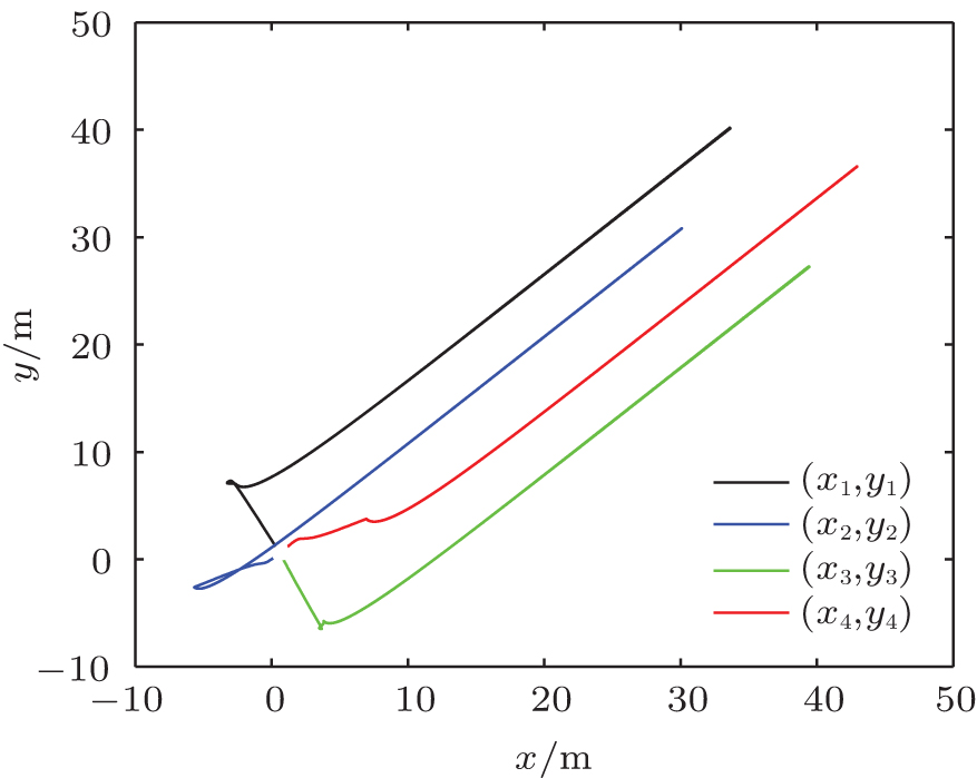	Fig.  3. Agents’ trajectories in the constant velocity case.

Fig.  4.

	Figure Option ViewDownloadNew Window
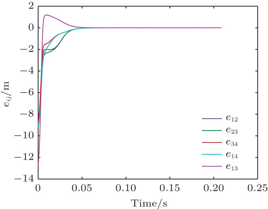	Fig.  4. Inter-agent distance errors for (i, j) ∈ ℰ in the constant velocity case.

Fig.  5.

	Figure Option ViewDownloadNew Window
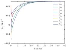
	Fig.  5. Agents’ velocities in the constant velocity case.

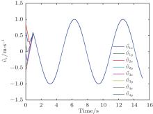
For the time-varying desired velocity case, let v_d(t) = cos (t). Figure  6 shows that the agents can achieve the formation asymptotically. Figure  7 describes the inter-agent distance errors which converge to zero. Figure  8 shows the velocities of all the agents which converge to the given time-varying velocity v_d(t) = cos (t).

Fig.  6.

	Figure Option ViewDownloadNew Window
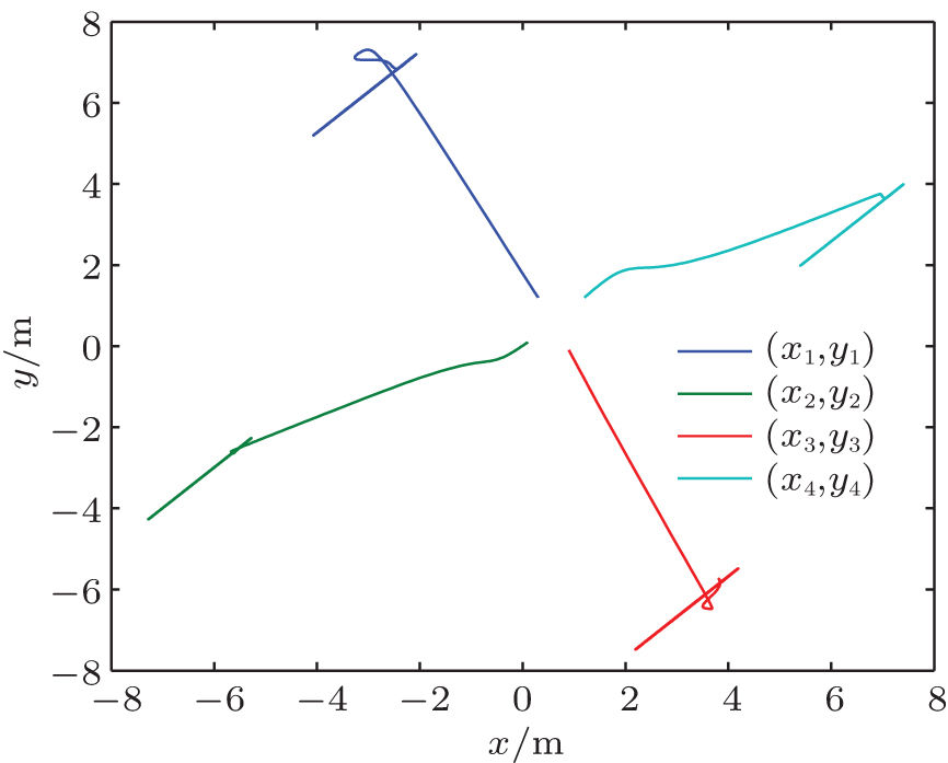	Fig.  6. Agents’ trajectories in the time-varying velocity case.

Fig.  7.

	Figure Option ViewDownloadNew Window
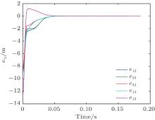
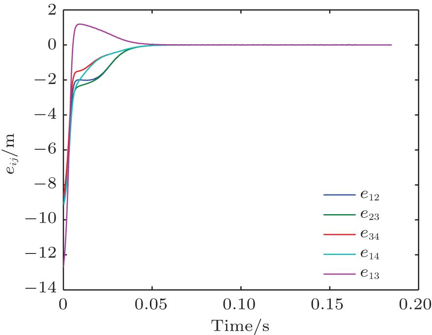	Fig.  7. Inter-agent distance errors for (i, j) ∈ ℰ in the time-varying velocity case.

Fig.  8.

	Figure Option ViewDownloadNew Window
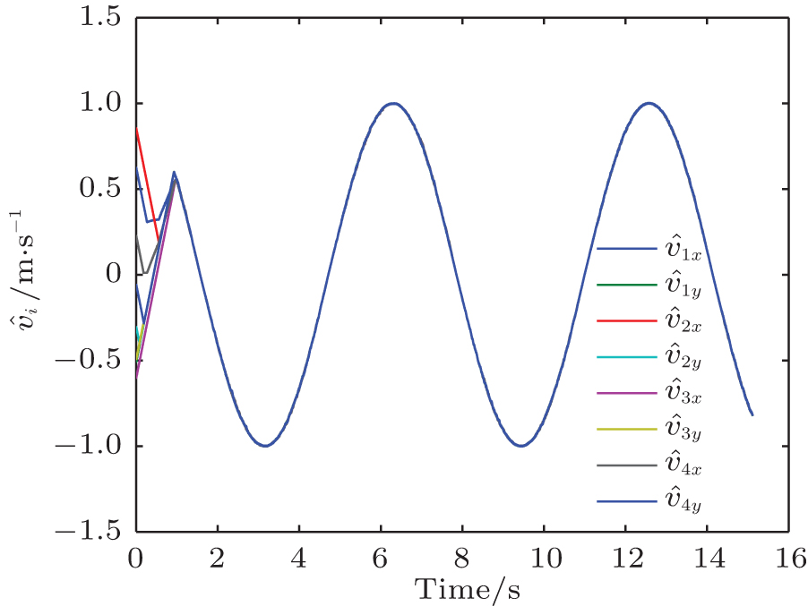	Fig.  8. Agents’ velocities in the time-varying velocity case.

In this paper, the distributed tracking problem of a minimally and infinitesimally rigid formation has been investigated. Two control algorithms have been designed to stabilize the inter-agent distances while allowing the formation to follow a constant or a time-varying velocity. In both cases, the desired trajectory velocity is assumed to be available to a subset of the agents. Distributed estimators have been constructed for each agent to estimate the desired velocity. The estimates are further employed to construct the control inputs of the agents where the rigidity matrix plays a central role. It has been proven that both the formation error and the estimator error can converge to zero. Finally, numerical examples have been proposed to verify the derived results.