
A study of the early warning signals of abrupt change in the Pacific decadal oscillation
[Wu Hao†a), b)  , Hou Wei
b) , Yan Peng-Chengb), c) , Zhang Zhi-Senb), c) , Wang Kuod) ]
, Hou Wei|
|


†Corresponding author. E-mail: wuhaophy@163.com
*Project supported by the National Natural Science Foundation of China (Grant Nos. 41175067 and 41305056), the National Basic Research Program of China (Grant No. 2012CB955901), the Special Scientific Research Project for Public Interest of China (Grant No. GYHY201506001), and the Special Fund for Climate Change of China Meteorological Administration (Grant No. CCSF201525).
In recent years, the phenomenon of a critical slowing down has demonstrated its major potential in discovering whether a complex dynamic system tends to abruptly change at critical points. This research on the Pacific decadal oscillation (PDO) index has been made on the basis of the critical slowing down principle in order to analyze its early warning signal of abrupt change. The chaotic characteristics of the PDO index sequence at different times are determined by using the largest Lyapunov exponent (LLE). The relationship between the regional sea surface temperature (SST) background field and the early warning signal of the PDO abrupt change is further studied through calculating the variance of the SST in the PDO region and the spatial distribution of the autocorrelation coefficient, thereby providing the experimental foundation for the extensive application of the method of the critical slowing down phenomenon. Our results show that the phenomenon of critical slowing down, such as the increase of the variance and autocorrelation coefficient, will continue for six years before the abrupt change of the PDO index. This phenomenon of the critical slowing down can be regarded as one of the early warning signals of an abrupt change. Through calculating the LLE of the PDO index during different times, it is also found that the strongest chaotic characteristics of the system occurred between 1971 and 1975 in the early stages of an abrupt change (1976), and the system was at the stage of a critical slowing down, which proves the reliability of the early warning signal of abrupt change discovered in 1970 from the mechanism. In addition, the variance of the SST, along with the spatial distribution of the autocorrelation coefficient in the corresponding PDO region, also demonstrates the corresponding relationship between the change of the background field of the SST and the change of the PDO.
A large number of studies[1, 2] have shown that the evolution of the climate system does not always advance gradually, and it is likely to change from one relative steady state to another within a short time. This change is known as an abrupt change of the climate system, which occurs on a different time scale.[3] An abrupt climate change will have a significant influence on social politics and economic environment, [2, 4, 5] as well as on social economic development and human life. Therefore, it is of vital realistic significance and scientific value to study[6, 7] the mechanism of an abrupt climate change, as well as its predicting technology and the theory for the abrupt climate changes that occurred in the 1920s, late 1970s, and early 1980s. At present, studies regarding the abrupt changes of climate systems have mainly focused on the detection of the abrupt change of climate and the explanation of its formation mechanism.[8– 17] There are currently few studies regarding the early warning signals of a system’ s abrupt change. The study of the identification and capture of the early warning signals of an abrupt change can further reveal the nature of an abrupt climate change, and thereby provide a scientific basis for the early warning forecast in the cases of catastrophic abrupt climate change accidents.
The phenomenon of abrupt change exists extensively in the natural world, particularly in complicated chaotic systems which often encounter changes among different states during an orderly evolution, and these changes are sometimes significant or even disastrous.[18, 19] The climate system always evolves first near a certain critical threshold, before the occurrence of an abrupt change, and the system will experience an abrupt change during the disturbance of a minor event. Therefore, some characteristics of the system, which are closest to critical threshold, can be regarded as early warning signals of an upcoming abrupt change of the system.[2]
Some major difficulties in today’ s weather forecasting include how to determine whether the climate system is approaching a critical point, and how to find the early warning signal before the occurrence of an abrupt change. In recent years, research results have shown that[20– 22] the phenomenon of a critical slowing down has important potential for revealing whether a complex dynamical system is approaching a critical catastrophe. This critical slowing down is a concept of statistical physics. It indicates that the system will approach a critical point before the dynamic system has changed from one phase state to another. In particular, a scattered fluctuation phenomenon conductive to the formation of a new phase state will occur at the critical points. This type of scattered fluctuation phenomenon shows not only an increasing fluctuation amplitude but also the longer duration of the fluctuation, the slow recovery rate, and the small recovery capability, which is referred to as the slowing down.[23] When a system approaches a critical point, the current state usually becomes unstable and transits into another state. Therefore, the recovery rate of the system disturbance slows during this time. In 2009, Marten Scheffer et al.[20] pointed out that the phenomenon of critical slowing down will lead to three possible early warning signals when the system approaches to its critical threshold. These signals are a slow recovery rate of disturbance, an increasing autocorrelation coefficient, and an increasing variance. This provides new thoughts for the forecasting of abrupt climate changes. Yan et al.[24] applied the theory of critical slowing down to the research of the precursory early-warning signal for the Wenchuan earthquake of 2008, and successfully determined the early-warning signal through the change of the water radon concentration prior to the earthquake. Wu et al.[25] and Tong et al.[26] applied the theory of critical slowing down to the research of the early warning signal of abrupt climate change and conducted research regarding the effectiveness and applicability of this method to various data in different areas. On this basis, research regarding the climate background field when a system approaches to a critical point will provide more evidence for the abrupt change mechanism of a single meteorological factor.
The Pacific decadal oscillation (PDO) is a type of strong climatic variability signal on a decadal time scale. It is also one of the signals with the strongest and most important global inter-decadal variability. On one hand, because the PDO is a disturbance super-imposed on the change of a long-term climate trend, it can cause the inter-decadal variation of climate in the Pacific and Pacific Rim. On the other hand, the PDO is also an important background of inter-annual variability, which plays an important role in the inter-annual variation. Therefore, research on the PDO is of vital significance for understanding climate variability in China or even throughout the world. Research[27– 29] has shown that the PDO has a good correlation with the Pacific SST and Nino phenomenon. Xiao and Li’ s research[7] also showed that the SST in the PDO region displayed inter-decadal variations, which is an important factor in the inter-decadal abrupt change of the global SST field. Research on the early warning signals of the PDO abrupt changes and its intrinsic system property, in combination with the theory of the critical slowing down, will potentially reveal the change law and the influence of the PDO system. The climate system is a complicated nonlinear dynamic system, [4, 30] and the Lyapunov exponent is an important physical quantity which indicates whether one system is in a regular motion or a chaotic motion. Therefore, research on the climate system using the Lyapunov exponent will show its potential application prospects.[31] Chen et al., [31] and Ding and Li[32] used the nonlinear local Lyapunov exponent to develop the research on the predictability of the atmospheric system. The present research provided new thoughts for the research of predictability. This study tests the early warning signal before an abrupt change of the PDO based on the phenomenon of critical slowing down, and uses the nonlinear Lyapunov exponent to theoretically verify this signal. This study also discusses the inherent property of a system before and after the occurrence of an abrupt change (near the critical point) by analyzing the largest Lyapunov exponent (LLE) at different times. Finally, this study analyzes the spatiotemporal variation of the SST in a corresponding area of the PDO, along with researching the relationship between the early warning signal of the PDO’ s abrupt change and the background field of the SST. This study also provides a certain experimental basis for the extensive application of the phenomenological method of the critical slowing down.
The data used are the monthly PDO index and the SST for 1961– 2010, which are published on the website of the National Oceanic and Atmospheric Administration (NOAA). In this paper, the SST data have a resolution ratio of 2° × 2° , selecting 20° N– 60° N, 140° E– 120° W; i.e., the covering range of the PDO model. In the actual calculation, the years from 1981 to 2010 are taken as the reference climate state, and the anomaly of original observation data is used as a reference climate state for a calculation sequence.
(i) Variance is the characteristic value that describes the extent of deviation of data in samples from the mean x̅ , denoted by s2, and s is the standard deviation. The computational formulas are, respectively, as follows:

where xi denotes the i-th data, and n is the number of data in samples.
(ii) The autocorrelation coefficient is a statistic describing the correlation of the same variable at different times. An autocorrelation coefficient with a lag length of j is denoted as c(j). The autocorrelation coefficients with different lag lengths can help to understand the relationship between the information at the current time and the information changes at the previous j time, thus judging the possibility of predicting xi+ j according to xi. For the variable x, the autocorrelation coefficient with the lag j is
where s is the standard deviation of the time series with size n and is determined from Eq. (2).
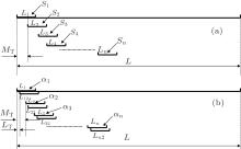
The variance and autocorrelation coefficient of the sequence are calculated through moving in the research in order to find the early warning signal of an abrupt change of the PDO index sequence. The specific method is shown in Fig. 1.
 | Fig. 1. We calculated the variance and autocorrelation coefficient by sliding the window. |
a) We calculated variance by sliding the window, L1, L2, L3, … , Ln … denote windows of the same length, S1, S2, S3, … , Sn … represent the variances of the corresponding windows, L is the total length of the sequence, and MT is the sliding step; b) we calculated the autocorrelation coefficient by sliding the window, L1(L12), L2(L22), L3(L32), … , Ln(Ln2)… represent windows of the same length, α 1 denotes the autocorrelation coefficients of L1 and the L12, α 2 denotes the autocorrelation coefficient of the L2, while L22, … the α n refer to the autocorrelation coefficients of the Ln and Ln2, LT represents the lag time, and L and MT have the same meaning as those in Fig. 1(a).
(iii) Relationship between the critical slowing down and the increased autocorrelation coefficient
A critical slowing down will tend to increase both the autocorrelation coefficient and the variance of the fluctuations in a stochastically forced system when the system approaches to a bifurcation at the threshold of the control parameter.[21, 22] It is assumed that there is a repeated disturbance of the state variable after each period Δ t (additive noise). Between disturbances, returning to equilibrium is approximately exponential with a certain recovery speed λ , which can be described with an auto-regressive model[21, 22, 33]

where xn is the deviation of the system variable from an equilibrium state, ε n is a random term with standard normal distribution, i.e., white noise in the system, and s represents the standard deviation. If λ and Δ t are independent of xn, then this model can also be written as a 1-order auto-regressive (AR(1)) process:

where the autocorrelation c = eλ Δ t is 0 for white noise and close to 1 for red noise.
The analysis of variance to AR(1) process leads to

Generally speaking, in the process where a system tends to its critical point, the recovery rate from small-amplitude disturbance will become increasingly slower.[33– 36] When the system is closer to the critical point, the recovery rate λ tends to 0, and the autocorrelation item c approaches to 1. Thus, the increased autocorrelation coefficient can be considered as an early warning signal that the system is approaching a critical point. In the calculation of this study, s represents the variance of the whole sequence, which is a constant value, while the Var value in Eq. (6) changes with the window size and moving step.
(iv) Lyapunov exponent
The Lyapunov exponent[37, 38] is an important physical quantity that is used to describe whether a system is in a regular motion or a chaotic motion. When at least one of the Lyapunov exponents of a system is positive, the system is considered to be chaotic. When all of the Lyapunov exponents of a system are negative, the system is considered to be convergent. Therefore, the LLE of a system is often calculated in order to determine whether the system is in a regular motion or a chaotic motion. The currently used methods for calculating the largest Lyapunov exponent of a chaotic time sequence includes the following:[39] the Nicolis method, the Jacobian method, the Wolf method (phase-space reconstruction method), the P-norm method, and the small-data method. Of these methods, the most common and widely used are the Wolf and small-data methods. This study adopts the Wolf method to calculate the LLE of the sequence. The specific operation steps of the Wolf method are described as follows.
The method of extracting the Lyapunov exponent from the time sequence of a single variable is based on the phase-space reconstruction of the time sequence. Wolf et al.[37] made an estimation of the Lyapunov exponent directly based on the evolution of the phase trajectory, phase plane, and phase volume, and so on. These methods are collectively referred to as the Wolf method, which is widely used to study the chaos and chaos time sequence predictions based on the Lyapunov exponent.
Assume that the chaos time sequence is x1, x2, … , xk, … , xN; the embedded dimension is m; and the time delay is τ . The reconstructed phase space will then be
In the actual calculation of this study, the embedded dimension m is 3 and the time delay τ is 12. Since the data used in this study are the monthly data, it is defined that the data of the current month has the smallest difference from the data of the corresponding month of the previous and following years. Take the initial point Y (t0), and assume that its distance with the nearest neighbor point Y0 (t0) is L0. Then trace the time evolution of these two points until the t1 time, when their spacing exceeds a certain value ε > 0, 


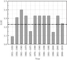
In this study, the LLE of the PDO index sequence at different time intervals is calculated through the Wolf method, which is used to determine the chaotic characteristics of the PDO index sequence at different times. The monthly data of the PDO index sequence during the period from 1951 to 2010 are selected, which totals 720. The LLE during the period of 1951 to 2010 is calculated to be 1.23 by using the Wolf method, and it is defined as the total LLE. Then, the LLE at each time interval (every five years) is further calculated and compared with the total LLE. The method of calculating the LLE at each time interval is as follows. First, a PDO time sequence (raw data minus the average and then divided by the mean square deviation) is standardized. Then, a random function is used to generate 1000 random arrays with a length of 60, followed by the averaging of these 1000 random arrays to obtain a random array with a length of 60. Then, the standardized treatment is realized. The calculated random number is used to gradually replace the value of the PDO index sequence at each corresponding time interval (gradually replace the values at the time intervals of 1951 to 1955, 1956 to 1960, … , 2001 to 2005, 2006 to 2010). The Wolf method is then utilized to calculate the LLE of the new sequence. The LLE of the PDO sequence is obtained at each time interval through the described replacements. The LLE reflects the chaotic characteristics of the system. It is determined that a larger exponent value will lead to stronger chaos characteristics.
The climate system experienced an abrupt change on a global (planetary) scale in the late 1970s and early 1980s. Simultaneously, the cold and warm phase positions of the PDO experienced an abrupt transition at approximately the year 1976.[7, 13, 40, 41] With regard to this abrupt change, this study analyzes the early warning signals of the abrupt change based on the principle of a critical slowing down, and uses the Lyapunov exponent to analyze the chaos characteristics of the PDO at each time interval, in order to evaluate the early warning signals. Finally, starting from the background field of SST (SST distribution of the PDO model), the relationship between the early warning signal of an abrupt change of the PDO and the background field of the SST is investigated.
Figure 2 shows the information of the PDO index sequence, PDO has obvious inter-decadal variations. The research results[7, 13, 40, 41] show that the cold and warm phase positions of the PDO experienced an abrupt transition (abrupt change) in 1976. The movement average trend line in Fig. 2 also illustrates that the phase position of the PDO before 1976 was at a cold phase position, and immediately changed to a warm phase position after 1976. Therefore, the PDO experienced a transition from cold to warm phase positions in 1976. This study mainly discusses the early warning signal of this abrupt change in 1976, retains the sequence before the abrupt change in 1976, and calculates the variance of the sequence, such as the length of parameter L, which is 312 months (monthly data within 1951 to 1976) before the abrupt change, and the autocorrelation coefficient in order to determine the early warning signal of an abrupt change, as shown in Fig. 1.
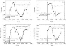
Figure 3 shows the early warning signals of the PDO index with different windows and moving step lengths. Figure 1 shows the variances of the moving calculation sequence and the autocorrelation coefficient, as well as the selection of the window moving and step length. For the purposes of this study, L1, L2, L3, … , Ln … , respectively, include 60 months (5 years) and 120 months (10 years). Similarly, L1(L12), L2(L22), L3(L32), … , Ln(Ln2)… also, respectively, include five years and 10 years. The moving step length MT is taken to be 1 month, while the lag time LT is taken to be 1 month. Figures 3(a) and 3(b) show the variance signals of the PDO index sequence. The moving step length (MT as shown in Fig. 1) indicates that the sequence with the selected window size would slide backwards by a fixed step length in order to obtain a new sequence, and then the variance of this new sequence could be calculated. The arrows in Figs. 3(a) and 3(b) show that the variance started to increase gradually around the year 1970 (figure 3(a) shows 1970, while figure 3(b) shows 1969). It can thus be known from the above theoretical analysis that the critical slowing down causes the lower internal change rate of the system, and the system’ s state at any time is very similar to its previous state. Therefore, the autocorrelation coefficient tended to be 1, and the variance according to Eq. (6) tended to be infinity. In principle, the critical slowing down reduces the system’ s ability to track the fluctuation and has an opposite effect on the variance. The phenomenon of critical slowing down, for example, the variance increase occurs when the climate system approaches to its critical point, can be regarded as an early warning signal for an abrupt change of the climate system, or as an early warning signal for the PDO’ s abrupt change which occurred around 1970. Therefore, it can be seen that the interval between the occurrence time of the early warning signal for the PDO’ s abrupt change and the occurrence time of an abrupt change is six years. This is a good indicator for climate predictions of a future abrupt change.
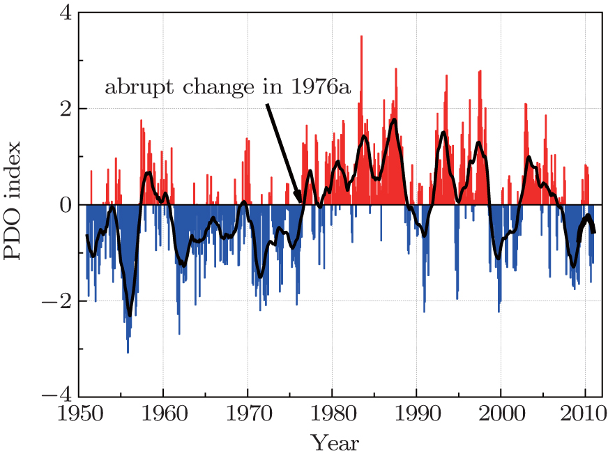 | Fig. 2. Curves of PDO index sequence changing with time (The bars represents the value of the PDO index: red for positive, blue for negative; and, a black curve for the trend information extracted from moving average). |
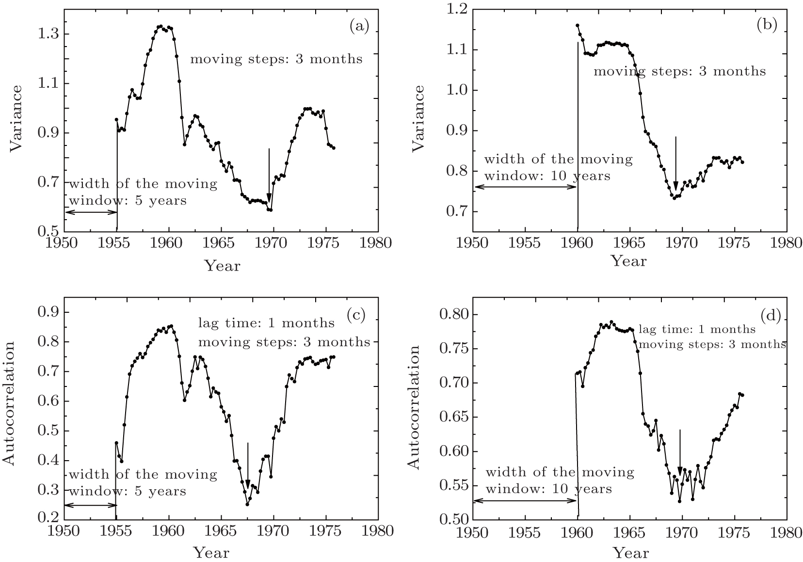 | Fig. 3. Critical slowing down phenomena in different window lengths and different sliding steps of PDO index, showing the signal of variances in (a) 5-year and (b) 10-year window lengths, and the signals of autocorrelation coefficient in (c) 5-year and (d) 10-year window lengths. |
Figures 3(c) and 3(d) show the autocorrelation coefficient detection of the PDO index sequence. It may be noted that the lag time (LT as shown in Fig. 1) and the moving steps (MTs as shown in Fig. 1) have different meanings in Figs. 3(c) and Fig. 3(d). The lag time refers to the original sequence, where the selected window size will be lagged for a selected step length to obtain another sequence with the same length, and to calculate the correlation (which is its own lag correlation) between the obtained sequence and the previous sequence. However, the moving step is the same as that of the variance signal. The arrows in Figs. 3(c) and 3(d) show that the autocorrelation coefficient starts to increase gradually (figure 3(c) shows 1967, while figure 3(d) shows 1970), the critical slowing down causes the lower internal change rate of the system, and the system’ s state at any time is very similar to its previous state. Therefore, the autocorrelation coefficient will tend to be 1. The phenomenon of the critical slowing down, such as the variance increase, increase of the autocorrelation coefficient, etc. when the climate system approaches to its critical point shows that the climate system will experience an abrupt change. Therefore, we can conclude that the early warning signal occurred in, approximately, 1970. We then determine that the time of early warning signal, which is discovered through the variance and autocorrelation coefficient, is the same. This further demonstrates the feasibility of finding the early warning signal of an abrupt change on the basis of the phenomenon of the critical slowing down.
Following the comparison of Figs. 3(a) and 3(b) with Figs. 3(c) and 3(d), it is easily determined that the different window sizes and moving steps would have an influence on the stability of the results. When the data volume is fixed, the larger window size and longer moving step mean that result is more stable. It is also more convenient to find the early warning signal of the abrupt climate change. References [25], [26], and [42] contain a detailed description regarding the influences of the window size and moving step on the stability results and the relevant research on the identification of the spurious signal. For example, when the data volume is fixed, the larger window size and longer moving step give a stabler result. Different lag steps with the same window also influence the result, and the selection of the window and lag step makes the signal disappear, and also influences the signal stability.
The preceding sections of this study test the early warning signal of the PDO abrupt change based on the phenomenon of the critical slowing down. However, the chaos characteristics and source of the early warning signal of the system approaching to its critical point are still a problem that urgently needs to be solved. The Lyapunov exponent is an important physical quantity which reflects whether the system is in a regular motion or a chaotic motion. Therefore, the LLE at each time interval should be calculated in order to investigate the intrinsic nature of the system, and to study its chaos characteristics.
Figure 4 illustrates the LLEs at each time interval and the total LLE of the PDO. It can be seen from Fig. 4 that the total LLE is 1.23 > 0, which indicates that the PDO system at this time interval is chaotic. It is found that a larger LLE value will make the chaotic characteristics of the system stronger. Only the LLEs within the time intervals of 1951– 1955, 1971– 1975, and 1996– 2000 are smaller than the LLE of the total sequence. We can obtain the specific calculation method of the LLE at each time interval by using the above theory. The random array replaces the original sequence at each time interval, and makes the LLE smaller, which means that the chaotic characteristics of the original sequence at these three time intervals are stronger. For example, the chaotic characteristics at the time intervals of 1951– 1955, 1971– 1975, and 1996– 2000 are stronger. The abrupt climate change refers to a phenomenon[1] where the climate crosses through a critical threshold and transits from one stable state (or a stable and continuous change trend) to another stable state (or a stable and continuous change trend). Through a comparison of the several time intervals between before and after 1976, in combination with the analysis of Figs. 2 and 4, the LLE during the period from 1956– 1970 is found to be positive. That is to say, the chaotic characteristics of the original sequence during this time interval is weaker. Similarly, the chaotic characteristics of the original sequence is stronger at the period of 1971– 1975, and weaker at the period of 1976– 1995. This means that the original sequence enters into a chaotic state from 1971 to 1975. Therefore, the phenomenon of a critical slowing down could be detected within this time interval, as could the phenomenon of early warning signal. Similarly, the chaotic characteristics of the original sequence are also stronger during the periods of 1951– 1955 and 1996– 2000. By comparing with the PDO index sequence shown in Fig. 2, it can be determined that the PDO transits from a cold phase to a warm phase position in, approximately, 1960 and 2000. Therefore, the chaotic characteristics of the original sequences at intervals of 1951– 1955 and 1996– 2000 are stronger. The conclusion that the PDO experiences an abrupt change during the years of 1960 and 2000 has been demonstrated in previous studies.[1, 7, 13, 43] However, no consensus has been reached for these two abrupt changes, as has been reached for the abrupt change in 1976, due to the consideration of the data length and the duration of time which has passed. In the same way, the early warning signal of the PDO’ s abrupt change during 2000 can be obtained by calculating the variance and autocorrelation coefficient of the sequence. However, the early warning signal of the abrupt change in 1960 cannot be found by using the above method, due to problems with the data length and the moving window (figure omitted).
 | Fig. 4. The LLEs of PDO index in each time period and total time series (The bars represent the LLEs of the PDO index in each time period, thick black dotted line is for the LLE of the total series). |
Based on the above factors, the LLE can successfully reflect the inherent chaotic characteristics of the PDO system and the changes of the chaotic characteristics shown at the different time intervals, thus providing the theoretical basis for the detectability of an early warning signal. In addition, the LLE further validates the feasibility of regarding the phenomenon of a critical slowing down as an early warning signal of an abrupt change.
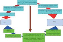
The PDO is a type of long-term existing Pacific climate change model. The PDO index of the United States National Climatic Data Center is expanded and reconstructed on the basis of the SST field of the NOAA, and the empirical orthogonal function (EOF) decomposition is conducted after removing the global warming trend in the SST field in the north of Pacific at 20° N. Its first principal component is defined as the PDO index.[27, 44] Therefore, the early warning signals of the PDO’ s abrupt change should be further studied from the aspect of the background field of SST. Figure 5 shows the relationship between the phenomenon of the critical slowing down caused by the PDO’ s abrupt change and the SST change rate in the corresponding areas.
 | Fig. 5. Relation among the SST, increased autocorrelation, and increased variance of PDO index. |
It can be concluded that the early warning signals of these two phenomena of critical slowing down (increase of autocorrelation coefficient and increase of the variance) before an abrupt change of the PDO occur at the same time. The increase of the autocorrelation coefficient of the PDO index means that the transition of the PDO between the positive and negative phase positions is more regular. For example, the spatial distribution-type change of SST in the area is more regular. Therefore, the change of SST at each lattice point of the area is also more regular, and the autocorrelation coefficient of SST change at each lattice point is also increased. The autocorrelation coefficient probability distribution diagram is given for the SST at each time interval to represent the autocorrelation coefficient of the sequence at each lattice point of the space. The characteristics of the increase of the autocorrelation coefficient of SST indicate a left advertence in the autocorrelation coefficient probability distribution diagram, and its peak value appears to be large.
In the same way, the increase of the PDO index variance indicates the increased change amplitude of the PDO phase position. For example, it transits from an obvious positive (negative) phase position to an obvious negative (positive) phase position. This also indicates the increased change amplitude of the spatial distribution pattern of the SST in the area, or the increased SST change amplitude at each of the lattice points of the area. Therefore, the variance of the SST change at each lattice point also increases, while the variance difference of the SST in the corresponding area decreases (the change rate of positive and negative phase position of the SST was synchronous). This is also reflected by the distribution diagram for the SST variance coefficient probability rate at each time interval, and its probability distribution rate indicates a centralized probability distribution and a narrow value range.
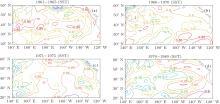
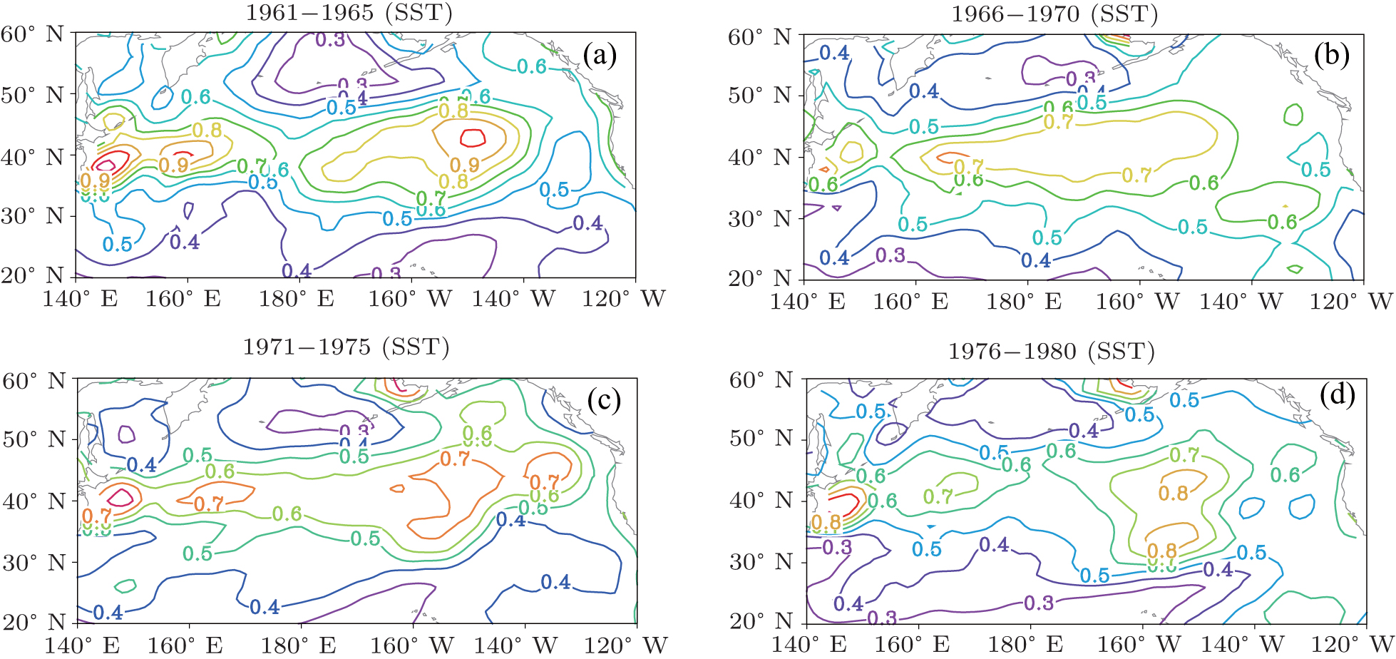
 | Fig. 6. The Distributions of the autocorrelation coefficient of the SST. |
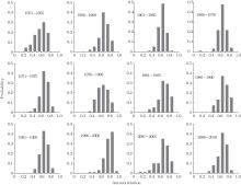
Figure 6 shows the spatial distribution diagrams for the autocorrelation coefficient (the lag time of the autocorrelation coefficient of the SST was − 1 in this study; i.e., lagging for one month, which corresponds to the autocorrelation coefficient calculation of the PDO) of the SST at time intervals of 1966– 1970, 1971– 1975, 1976– 1980, and 1981– 1985. This study focuses on the early warning signals of the PDO’ s abrupt change before and after 1976, thus only these four time intervals are selected for analyses. Similarly, the spatial distribution diagram could also be made for the autocorrelation coefficient at each time interval. It is known from the analysis in Fig. 5 that the autocorrelation coefficient of the SST in the corresponding area also increases if the autocorrelation coefficient of the PDO index augments. It may be concluded from Fig. 6 that the autocorrelation coefficient of the SST at the time interval from 1971 to 1975 is larger than that at the other time intervals. In other words, there is a critical slowing down phenomenon when the autocorrelation coefficient is increased, but such a trend is not obvious. Therefore, in order to explain this problem, further analysis should be conducted by using the probability distribution diagram for the autocorrelation coefficient at each time interval, as shown in Fig. 7. In Fig. 5, if the autocorrelation coefficient of the PDO index sequence is increased, then the autocorrelation coefficient of the corresponding SST is also increased. Moreover, the probability distribution diagram for the autocorrelation coefficient of SST shows a left advertence, and its peak value is large. Comparisons among these characteristics and the creation of the contrastive analysis on the probability distribution diagram for the autocorrelation coefficient at each time interval are shown in Fig. 7 (the autocorrelation coefficient probability distribution in the total time interval of 1951– 2010 is close to the normal distribution). It can be easily determined that the characteristics at the time intervals of 1971– 1975 and 1996– 2000 comply with the judgment basis, which illustrates that in the SST during 1971– 1975 there appears a phenomenon of a critical slowing down. Therefore, these results demonstrate that the reliability and reasonability of an early warning signal for an abrupt change in 1976 of the PDO system can be found in 1970 from the aspect of the background of SST. In the same way, the phenomenon of a critical slowing down occurs between 1996 and 2000, and this can also be regarded as the early warning signal of an abrupt change[7, 43] which occurs around the year 2000. From the above discussion, the phenomenon of a critical slowing down, such as the increase of the autocorrelation coefficient occurring before the PDO’ s abrupt change, can be regarded as an early warning signal of its abrupt change. Such a phenomenon shows a good correlation with the SST in its corresponding area. The analysis on the autocorrelation coefficient from the background field of the SST also demonstrates the reliability and reasonability of the determined early warning signals.
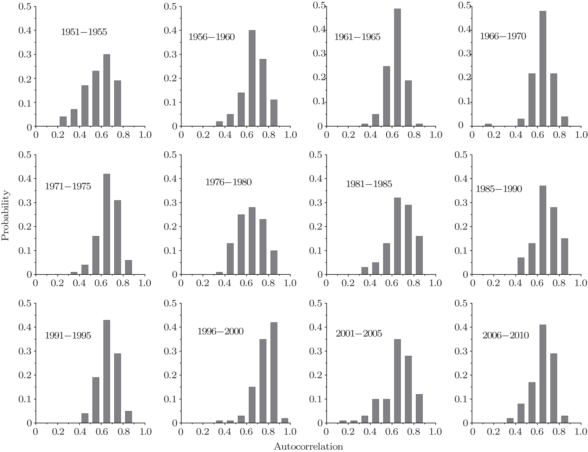 | Fig. 7. Probability distributions of the autocorrelation coefficient of the SST in each time period. |
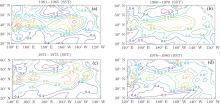
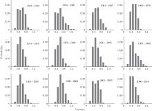
Like the analysis of autocorrelation coefficient, the relationship between the early warning signal of the PDO’ s abrupt change which is based on the increased variance and the variance of SST in the corresponding area, will be discussed below from the point of view of variance. Figure 8 shows the distribution diagrams for the variance of SST in the four time intervals. In accordance with the analysis shown in Fig. 5, it is known that if the PDO index sequence exhibits the phenomenon of a critical slowing down, such as a variance increase, then the SST in the corresponding area of the PDO will show an increased change rate, and the variance differences of SST in the corresponding area will be reduced. Using the comparative analysis of Fig. 8, it can be found that the variance difference of the SSTs in the area from 1971 to 1975 is smaller, and the SST model in the area is relatively stable. Figure 9 shows the probability distribution diagrams for the variance of SST at each time interval. In accordance with the aforementioned theory and the analysis shown in Fig. 5, it is known that if in the PDO system there occurs a phenomenon of a critical slowing down, such as a variance increase, then the probability distribution of the variance of the SST in the corresponding area will show a concentrated distribution (ensuring that the change rates of the positive and negative phase positions of the SST are synchronous), which means that the value range of its probability distribution diagram is relatively narrow. In accordance with this judgment basis, and by making a comparative analysis on the distribution characteristics at each time interval, as shown in Fig. 9, we can easily find that the distribution characteristics at the time intervals of 1966– 1970 and 1971– 1975 meet the requirements. This indicates that in the SST there occurs a phenomenon of a critical slowing down at this time, and it also
 | Fig. 8. Distributions of the variance coefficient of the SST. |
 | Fig. 9. Probability distributions of the variance coefficient of the SST in each time period. |
The above-mentioned research is performed by using the annual and monthly continuous SST data. Although the anomaly treatment has been made for the sequence, its sequence still has the inter-decadal, inter-annual, and seasonal change trends and it cannot reflect the inter-monthly autocorrelation and variance characteristics of SST. Therefore, the monthly change trend of the SST is obtained through a low-pass filtering treatment, before calculating the autocorrelation coefficient and variance coefficient of SST. In this study, the sequence without a low-pass filtering treatment is also calculated (figure omitted), and the result is very similar to that given earlier in this paper, which means that the change of SST is dominated by a high-frequency seasonal change signal. Therefore, the phenomenon of a critical slowing down which occurs before the PDO’ s abrupt change can be regarded as the early warning signal of its abrupt change, and this phenomenon has a good correlation with the SST in its corresponding area. The analysis regarding the autocorrelation coefficient from the background field of SST also demonstrates the reliability and reasonability of the determined early warning signal.
In this study, we analyzed the physical basis and statistical significance of the phenomenon of a critical slowing down on the basis of the PDO index data. We then discussed the early warning signal of an abrupt change of the PDO system which occurred in the late 1970s and early 1980s (1976) by using the principle of a critical slowing down. In this study we also used the Lyapunov exponent to investigate and analyze the chaotic characteristics of a PDO index sequence at each time interval, which, to a certain extent, demonstrates the possible reason for an early warning signal of a PDO abrupt change from the viewpoint of a mechanism. Finally, starting from the background field of SST, in this study we explored the relationship between the early warning signal of a PDO abrupt change and SST in the corresponding period. We then drew the following conclusions:
i) The phenomenon of a critical slowing down observed before a complicated dynamic system experiences an abrupt catastrophe may be the early warning signal indicating that the catastrophe will occur. The PDO research conducted by using the variance and autocorrelation coefficient, which can reflect the phenomenon of a critical slowing down, not only deepens the understanding of the fluctuation information in the precursory observation data but also provide a new method of determining the abnormal reliability. A critical slowing down phenomenon occurred six years prior to the PDO’ s abrupt change, such as the increase of variance and autocorrelation coefficient, which indicates the feasibility of an early warning signal of an abrupt change based on the phenomenon of a critical slowing down.
ii) Through the research of the chaotic characteristics of the PDO at each time interval by using LLE, it is found that the time intervals of 1951– 1955, 1971– 1975, and 1996– 2000 show the strongest chaotic characteristics. This indicates that the system at these three time intervals is in a chaotic critical slowing down phase, and this could be used as the early warning signal of an abrupt change. Although this study mainly focuses on the early warning signal of an abrupt change of the PDO system in 1976, and shows that the strongest chaotic characteristics occur at the interval between 1971 and 1975, the correctness of the occurrence of an early warning signal of a critical slowing down in 1970 can be reasonably explained. In addition, the PDO system makes early warnings of two abrupt changes which are unknown, occurring in the early 1960s and 2000s, respectively, and provides data to support the common application of this method.
iii) Starting from the background field of SST, this study focuses on the relationship among the variance and autocorrelation coefficient of SST in the corresponding PDO area and the early warning signal of the PDO’ s abrupt change. The research results indicate that the variance and autocorrelation coefficient of the corresponding SST also experiences the same changes as both the abrupt change of the PDO system in 1976 and the increase of the variance and autocorrelation coefficient (early warning signal of an abrupt change) in 1970. The probability distribution diagram of the variance of the SSTs shows the characteristics of a narrow value range during 1971– 1975, and the autocorrelation coefficient probability distribution diagram of the SST shows the characteristics of a left advertence and large peak value from 1971 to 1975. Using the probability distribution diagrams for the variance and autocorrelation coefficient at each time interval of the SST, we can reasonably explain both the abrupt change of the PDO system in 1976, and the increase of the variance and autocorrelation coefficient (early warning signal of an abrupt change) in 1970.
In this study, we investigated the trend of the variance and autocorrelation coefficient of a sequence after removing the inter-decadal change, and then conducted the retrospective verification of the phenomenon of a critical slowing down before an abrupt change. The results show that the early warning signal of an abrupt change which is based both on the variance and the autocorrelation coefficient is very applicable to the PDO index data verification. This means that the phenomenon of a critical slowing down can be regarded as an early warning signal of a climate abrupt change. By analyzing the chaotic characteristics of the PDO system through using LLE, it is indicated that the PDO system was in a critical slowing down phase during 1971– 1975, which can reasonably explain both the abrupt change of the PDO system in 1976 and also the increase of the variance and autocorrelation coefficient (early warning signal of abrupt change) in 1970. Through the analysis on the background field of SST, it is determined that the background field of SST in the corresponding PDO area has a high correlation with the early warning signal time of the PDO’ s abrupt change. In general, although this research is a preliminary study on the early warning signal of an abrupt climate change, the phenomenon of a critical slowing down provides the possibility to improve the understanding of the precursory observation data, determines whether the anomaly approaches to a critical phase, and increases the catastrophe prediction level. Meanwhile, a reasonable explanation could be made from the aspect of a mechanism and a background field. The introduction of a critical slowing down theory into the research on the early warning signal of an abrupt climate change has great practical significance and scientific value for an in-depth understanding of abrupt climate change and finding the early warning signals of abrupt climate change. It also lays a foundation for the actual extensive application of this method.
It should be pointed out that the research of the PDO index data shows that the increase of variance and autocorrelation coefficient in the mechanics, caused by the phenomenon of a critical slowing down, is a possible early warning signal prior to the occurrence of an abrupt change, and a reasonable explanation was made from the aspect of a mechanism and background field. However, in fact the climate system is a very large and dissipative chaotic system, and the occurrence and prediction of abrupt change are very complicated. This research is still at a preliminary level, thus it is necessary to conduct further research on the space scope which occurs in the phenomenon of a critical slowing down before an abrupt change. The relationship between the phenomenon of a critical slowing down and the abrupt change strength of a climate, the quantitative analysis when regarding the increase of variance and autocorrelation coefficient, reflected by the phenomenon of critical slowing down, as the early warning signal before climate abrupt change, the reasonable analysis of the background field characteristics, etc., require further investigation.
| 1 |
|
| 2 |
|
| 3 |
|
| 4 |
|
| 5 |
|
| 6 |
|
| 7 |
|
| 8 |
|
| 9 |
|
| 10 |
|
| 11 |
|
| 12 |
|
| 13 |
|
| 14 |
|
| 15 |
|
| 16 |
|
| 17 |
|
| 18 |
|
| 19 |
|
| 20 |
|
| 21 |
|
| 22 |
|
| 23 |
|
| 24 |
|
| 25 |
|
| 26 |
|
| 27 |
|
| 28 |
|
| 29 |
|
| 30 |
|
| 31 |
|
| 32 |
|
| 33 |
|
| 34 |
|
| 35 |
|
| 36 |
|
| 37 |
|
| 38 |
|
| 39 |
|
| 40 |
|
| 41 |
|
| 42 |
|
| 43 |
|
| 44 |
|