
Magnetization plateaus and frequency dispersion of hysteresis on frustrated dipolar array
[Zhang You-Tian† ]
]
]
|
|


†Corresponding author. E-mail: ytzhang@smail.nju.edu.cn
Competings or frustrated interactions are common for condensed matter systems. In consideration of the effect of dipole–dipole interaction, the static properties of square lattice spin systems are investigated using the Wang–Landau algorithm. The dynamic hysteresis is also simulated using the Monte Carlo (MC) method. The step-like magnetization under a DC magnetic field and two distinct peaks in hysteresis dispersion under an AC magnetic field are observed. Then, the formation of the properties of the frustrated dipolar array are discussed.
Frustration is considered as a competition between interactions.[1] Hence, not all interactions can be satisfied in the system with frustration. As an example, an artificial, geometrically frustrated magnet can be conducted on an array of lithographically fabricated single-domain ferromagnetic islands.[2– 4] The islands can be arranged in a way that the dipole interactions create a two-dimensional (2D) analogue to spin ice.[5– 7] On a 2D manufactured lattice, the state can be visualized with magnetic force microscopy directly. The study on artificial spin ice can not only investigate many-body phenomena related to frustration, monopole-like excitations, and out-of-equilibrium thermodynamics in a material, but also contribute to the progress of new materials in novel spintronic devices.[8]
The fields from dipolar sources are formed by long-range interactions, thereupon the ordering in dipolar lattices depends on details of the geometry.[9] There are many kinds of artificial spin ice lattice structures. Shakti lattice, none of whose near-neighbor interactions is locally frustrated, does not directly correspond to any known natural magnetic material.[10, 11] Square lattice and kagome lattice form two key artificial spin ice geometries, namely elongated single-domain nanomagnets placed on the sites of a square lattice and the kagome lattice respectively. The interactions between the islands at a three-island vertex are equivalent in artificial kagome spin ice, while the interactions between nanoislands at a four-island vertex are not equivalent in square spin ice. Although properties of artificial spin ice are well described by short-range spin ice models (disorder and ice-like rules are satisfied), the magnetic structures and behaviors under external fields can depend on approximations made in the modeling of long-range interactions for some systems.[12] Square lattice is focused in this article.
The magnetic responses in magnetostatic fields and in alternating current magnetic fields for spin ice systems have different characteristics. The phenomenon of magnetization plateaus under stationary magnetic fields is common in frustrated systems.[13] Multi-step magnetization behaviors, which are believed to be generated by the non-equilibrium dynamics of frustrated spin systems, Shastry– Sutherland lattice, and kagome spin ice system for instance, are investigated by employing the Wang– Landau algorithm.[14, 15] When an alternating magnetic field is applied, due to the relaxation delay, the relationship between field strength (H) and magnetization intensity (M) is not linear in ferromagnetic system. A loop will appear due to the dynamic lag between input and output if the H– M relationship is plotted for all strengths of applied magnetic fields in one cycle. The dependence of the hysteresis loop area, as a function of the frequency of applied magnetic field, can be used to study the dynamics of spin reversal, which is known as the hysteresis dispersion. Investigations on the hysteresis dispersion, both simulatively and theoretically, are focused.[16– 18] This article will first introduce the model and simulation methods. Then the results of an investigation on the magnetization plateaus of square lattice are presented. At last, the hysteresis effect on the square lattice is studied using the Monte-Carlo method with extra focus on the frequency dispersion properties.
For this kind of square, frustrated dipolar array, its magnetization was analyzed with a stationary magnetic field applied and its hysteresis with an alternating magnetic field applied. In simulations, 16 × 16 square lattices, and periodic boundary conditions are used. On each lattice point, a spin is put and only two opposite directions each spin can point to. The coordinate system we choose is shown in Fig. 1. Considering the Zeeman energy, the nearest exchange interaction and the long-range dipolar interaction, the following Hamiltonian is used to describe the system
where H is the magnetic field applied; J is exchange interaction coefficient; D is dipolar interaction factor and rij ≡ ri − rj is the spatial vector between spins si and sj. These three interaction terms compete with one another. Because the magnetic structures may trap at some metastable states, an ideal approach is to employ the WLS algorithm.[19, 20] In the simulation, the modification factor ranges from e1 to 1.000000. If the data scattering was less than 20% of the average histogram over the whole energy space, the histogram was regarded as flat.
 | Fig. 1. The direction of x and y axes are (0, 1) and (1, 0). So, the directions of the spins at the vertices are (i)     |
The density of states (DOS) was calculated with the standard WLS first. The transition probability of a random walk from an event with energy E1 to that with energy E2 can be calculated according to the importance sampling rule of the WLS as follows:
Then, M will be recorded if the random walk visits event with energy E. We then get spectrum M(E) and magnetization can be calculated with the one-dimensional DOS g(E) by

Hysteresis dispersion of this system under alternating magnetic field and low temperature situation is investigated using the standard Metropolis Monte Carlo algorithm. The MC method is generally a way to simulate the thermal equilibrium state of the system with many degrees of freedom under certain external condition. The MC method is also employed to approach the response of a system in simulations where the external conditions are changing with time.[21, 22] More details of Monte Carlo simulation in this article are described as follows. We set J = − 1.5, D = 1, kB = 1, and |H(t)| = H0sinω t, where H0 is the amplitude of the magnetic field applied. Also, the angle between magnetic field and x axis is still chosen to be 56.31° , in which condition the hysteresis loop naturally exhibits the three-step character when low frequency magnetic field is applied. On a two-dimensional square lattice with periodic boundary condition, a spin is randomly chosen at each time step. Then we can calculate the energy difference (Δ E) of the system after and before flipping the spin. If exp(− Δ E/kBT) is bigger than a randomly chosen number between 0 and 1, the spin will be reversed. Before the field is updated in the next time step, one or more spins can be chosen randomly depending on the different frequencies of the magnetic field. In our simulation, frequency f = 1 refers that between two continuous steps updating the magnetic field, only one spin is chosen to attempt flipping. Ahead of applying magnetic field, we first decrease temperature from a certain value to low temperature. In each step of decreasing the temperature, 105 Monte Carlo steps are used to reach equilibrium. Then we begin to perform the introductory cycles (100 periods, without measurement). Next, we conduct measurement of the hysteresis loop with 600 points on it. It should be noted that we measure the projection of the total magnetization along the direction of magnetic field as M, and take mean value of 50 periods after introductory cycles for each point (M, H) on the final hysteresis loop. At last, we calculate the area (A) of the hysteresis loop. For different frequencies, we can get different areas correspondingly.
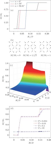
We applied the DC magnetic field along different directions. When the magnetic field is applied along x axis, the system reaches magnetic saturation directly. If the magnetic field is applied along angular bisector of x and y axes, the system will not reach magnetic saturation. As for other directions, a three-step M profile as the ground state can be observed which is caused by the competition between dipolar interaction and Zeeman energy. A suitable angle between magnetic field and x direction is chosen to be 56.31° , that is, the magnetic field component ratio of y and x is 1.5. The middle step is broader in this case. For three-step M– H profile, the ground states of each step are different as well as the energy. We track the magnetic structures of different magnetization intensities as shown in Fig. 2(b). Simulated M(H, T) profile (see Fig. 2(c)) is given on the condition that Hy = 1.5Hx, D = 1.0, J = − 1.5. Some of the section views reveal magnetizing curves at different temperatures as shown in Fig. 2(d).
 | Fig. 2. (a) Depictions of the M– H profile when magnetic field is applied along different directions. (b) The ground-state magnetic structures of different steps in the M– h curve. Panel (c) is the simulated result in the situation that Hy = 1.5Hx, D = 1.0, J = − 1.5. The angle α between magnetic field and x direction is 56.31° . Note that the magnetization is normalized by the saturated magnetization. |
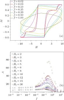
The dynamics of spin reversal can be characterized by the characteristic time (τ ). The shape and area of hysteresis are fully determined by the relative dominance between τ and f− 1.[17] From the perspective of classical relaxation, spin reversal has the characteristic time for given amplitude of the applied field. If the characteristic time is comparable to the periodicity of the field, then the system reaches the resonance and an extreme of hysteresis loop area is revealed. Usual hysteresis dispersion exhibits a single-peaked pattern due to the characteristic time of spin reversal.[23] If τ ≪ f− 1, then the spin reverses sufficiently in the system, and the quasi-static hysteresis shows relevant characters to the M– H curve under the constant magnetic field condition in our results. The peak of the hysteresis dispersion A(f) grows upwards and shifts rightwards gradually with increasing field amplitude H0 (see Fig. 3(b)). At high frequency, A(f) shows sufficient linearity in double-log plot with the slope − 1 (see Fig. 6(a)), which indicates A ∝ 1/f when the frequency is high.
 | Fig. 3. (a) Different hysteresis loops when different frequencies of magnetic field are applied with T = 0.1, H0 = 10. For the quasi-static hysteresis under H0 > 8 conditions, magnetic saturations, whose magnetic structures are the same as the third situation in Fig. 2(b), are always attained. (b) The peak of the hysteresis dispersion moves upwards and shifts rightwards gradually with increasing field amplitude H0. In addition, A ∝ 1/f can be obtained when frequency is high. |
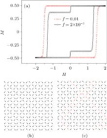
For quasi-static hysteresis under weak magnetic field, the steady magnetic structure changes when frequency range is at low levels (see Fig. 4). Two M > 0 steady states were observed in H0 = 2, f = 2 × 10− 5 situation and their magnetic structures are also tracked. The loop area decreases by forming new steady magnetic structures at the lower frequencies. This reveals that, with the decrease of frequency, the area gradually diminishes due to the diminution of coercive field until at a certain frequency, the sudden change of area occurs because of newly formed steady state with lower magnetization. Then the coercive field decreases little by little again till another steady magnetic structure with smaller magnetization arises. In this way, the loop area decreases with lower magnetic field frequencies.
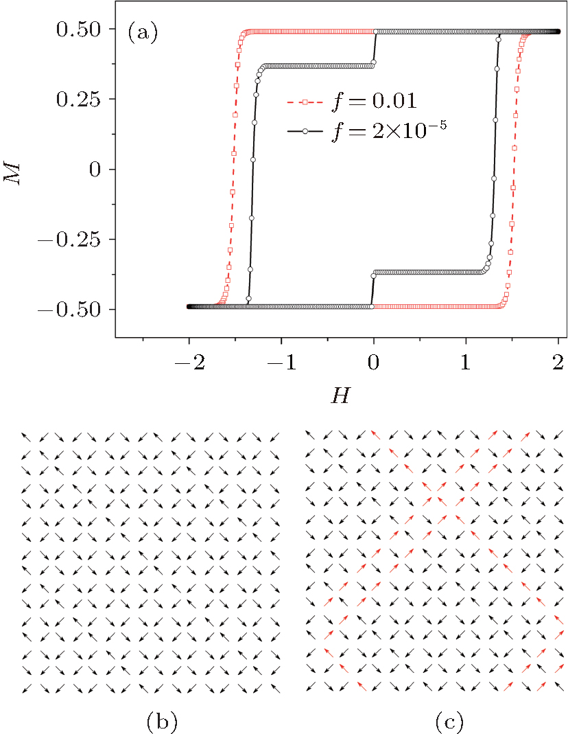 | Fig. 4. (a) For quasi-static hysteresis under H0 < 6 conditions, a new magnetic structure is revealed and the loop area gets smaller. Here, H0 = 2. Panels (b) and (c) are the magnetic structures of high and low magnetization states (two steady states with M < 0) under H0 = 2 and f = 2 × 10⁵ respectively. |
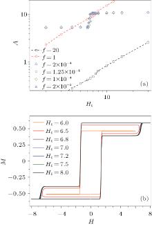
At low frequencies, as is shown in Fig. 5(a), the loop areas have similar dependance on H0 (amplitudes of applied AC magnetic fields). Meanwhile, a leap between H0 = 6 and H0 = 8 at low frequencies is evidently observed. This hints that there is a range of transition magnetic field amplitudes between weak and strong magnetic field. Within the range of transition magnetic field amplitudes, we investigate the shape variation of hysteresis loops at certain low frequency (f = 10− 4 here). The system has one M > 0 steady magnetic structure with H0 = 6 and has two M > 0 steady magnetic structures with H0 = 8. As magnetic field amplitude increases from H0 = 6 to H0 = 8, one magnetization intensity of steady magnetic structure splits into two values (see Fig. 5(b)). Also, this splitting behavior is consistent with the magnetization properties in the DC magnetic field. Under low frequency strong field, the hysteresis loop in the first quadrant is similar to the step-like magnetization in the DC field which is described earlier in this article. It is reasonable to regard the DC field condition as AC field situation with frequency f → 0.
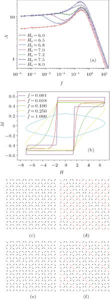
The hysteresis dispersion A(f) is then studied when the amplitude of the applied magnetics field is between 6 and 8. Two distinct peaks are observed (see Fig. 6(a)). The main peak on the right side is dominantly related to the collective behavior of the spin reversal and the emerging peak on the left can be ascribed to the oscillation of monopoles.
 | Fig. 5. (a) A leap of the hysteresis area can be observed in low frequencies. (b) The shapes of hysteresis loops change with different amplitudes of magnetic fields applied at low frequencies (f = 10− 4 here). Only one steady state exists when H0 = 6, but, for larger amplitudes, two steady magnetic structures exist. |
We pay close attention to the formation of the valley in hysteresis dispersion A(f) intuitively. While there can be two steady magnetic structures when the amplitude of the applied magnetic field is 7, the magnetic structures and the corresponding magnetization intensity change with the frequency of the applied magnetic field. There is a magnetization intensity difference between the two steady magnetic structures; f = 0.001 is bigger than that of f = 0.018. Accordingly, tracking the magnetic structures, it is figured out that the magnetic structure of f = 0.001 changes more considerably. Bigger magnetization intensity difference enlarges the hysteresis loop area in f = 0.001 case. For f = 0.100, only one steady magnetic structure exists. But the loop area of f = 0.100 is still bigger than loop area of f = 0.018 due to the bigger intensity of the coercive field. Thus, A(0.001) > A(0.018) < A(0.100). More generally, within the range of this transition magnetic field amplitude, the intensity of the coercive field (especially for higher frequencies) and the magnetization intensity difference between the two steady magnetic structures (for lower frequencies) are the main factors to determine the area of the hysteresis loop. There is a certain suitable frequency to minimize the area of the hysteresis loop with smaller coercive field and magnetization difference, then a valley in hysteresis dispersion forms.
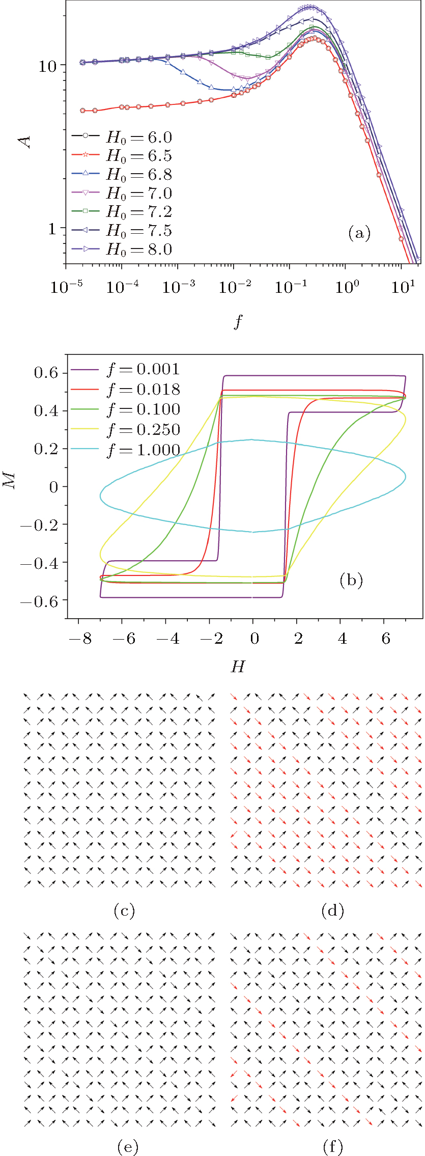 | Fig. 6. (a) Two peaks can be observed in the range of the transition magnetic field. (b) Different hysteresis loops under different frequencies of applied field when the amplitude of the magnetics field is 7. Panels (c)– (f) are the steady magnetic structures of high/low magnetization states. (c) f = 0.001, high magnetization magnetic structure; (d) f = 0.001, low magnetization magnetic structure; (e) f = 0.018, high magnetization magnetic structure; (f) f = 0.018, low magnetization magnetic structure. |
In this article, the responses of square spin ice to both static magnetic fields and alternating magnetic fields are discussed. When applying a static magnetic field in certain directions, a three-step M profile as the ground state is observed, which is in consistent with the hysteresis loop appeared as the stepwise character when low frequency alternating magnetic field is applied. The hysteresis dispersion of the square ice responses to alternating magnetic fields is then investigated. The hysteresis loop area is inversely proportional to frequency in the high frequency range. The hysteresis loop area is not varying continuously versus the magnetic field amplitude in the low frequency range. How the hysteresis loop area decreases when the frequency declines in alternating weak magnetic field is also explored. For transition amplitudes of applied magnetic fields, the formation of double peaks in hysteresis dispersion is investigated.
The author is grateful to Prof. J. M. Liu and Dr. Y. L. Xie from the Pulsed Laser Deposition Laboratory of Nanjing University for valuable discussions.
| 1 |
|
| 2 |
|
| 3 |
|
| 4 |
|
| 5 |
|
| 6 |
|
| 7 |
|
| 8 |
|
| 9 |
|
| 10 |
|
| 11 |
|
| 12 |
|
| 13 |
|
| 14 |
|
| 15 |
|
| 16 |
|
| 17 |
|
| 18 |
|
| 19 |
|
| 20 |
|
| 21 |
|
| 22 |
|
| 23 |
|