

A novel method of evaluating the lift force on the bluff body based on Noca’s flux equation
[Sui Xiang-Kun†a)  , Jiang Nan
a), b), c) ]
, Jiang Nan|
|


†Corresponding author. E-mail: xksui@lnm.imech.ac.cn
The influence of experimental error on lift force evaluated by Noca’s flux equation is studied based on adding errors into the direct numerical simulation data for flow past cylinder at Re = 100. As Noca suggested using the low-pass filter to get rid of the high-frequency noise in the evaluated lift force, we verify that his method is inapplicable for dealing with the dataset of 1% experimental error, although the precision is acceptable in practice. To overcome this defect, a novel method is proposed in this paper. The average of the lift forces calculated by using multiple control volume is taken as the evaluation before applying the low-pass filter. The method is applied to an experimental data for flow past a cylinder at approximately Re = 900 to verify its validation. The results show that it improves much better on evaluating the lift forces.
Unsteady aerodynamics of flapping wings is important for the future design of micro-air-vehicles (MAVs) at low Reynolds number flows.[1] Due to their small magnitudes, the lift forces on MAVs are difficult to experimentally measure by the extrinsic methods, such as the strain gauges, instead, the intrinsic methods are used in this case. For the steady cases, the Kutta– Joukowski (K– J) theorem is widely used to calculate the lift forces. While for the unsteady cases, the equations derived from the Navier– Stokes equations need to be used, [2– 8] such as the ones derived by Noca et al., [9– 12] because the K– J theorem is no longer valid.[13] Noca’ s equations are convenient for the Particle Image Velocimetry (PIV) measurement, since they only involve the velocities and their derivatives. However, the simplest expression is “ the flux equation” which requires information about the surfaces of the control volume and the body. In this paper, we will develop a novel method to calculate lift forces from experimental data by using the flux equation.
Several studies have been carried out to evaluate lift forces based on the flux equation, [11, 12, 14– 19] where they considered many factors which may introduce numerical errors in the computing process. Noca et al.[11, 12] studied the effects of time differencing schemes and domain sizes on calculating lift forces and suggested using the low-pass filter to get rid of the errors in results. Baik et al.[15, 16] and Sterenborg et al.[19] avoided the sensitivities of the flux equation to origin locations of the coordinate system and control volume contours in their experiments by using multiple origins or control volumes, while Ferreira et al.[17] and Zanon et al.[18] placed the origin location in the middle of the wake in their experiments.
The mentioned studies focused on how to deal with numerical errors, while the experimental errors in PIV measurements, which are also amplified in the computing process, have not attracted due attention. According to Noca’ s method, they caused high-frequency noises in lift forces. But in the present paper we verify that the low-pass filter is inapplicable in the lift forces calculated from the PIV dataset with 1% experimental errors even if the effect of numerical errors on calculating lift forces can be ignored, since the lift forces contain large low-frequency fluctuations which also need to be eliminated. The proposed novel method solves the problem by averaging the lift forces of multiple control volumes before using the low-pass filter.
The rest of this paper is organized as follows. In Section 2 the validation of the novel method is carried out. First, the lift forces are calculated by the flux equation using a direct numerical simulation (DNS) dataset for flow past cylinder at Re = 100. Then, an artificial error-added dataset is produced by adding random errors into the dataset to simulate a PIV result. Finally, the lift forces calculated by Noca’ s method and the novel method using the artificial dataset are compared with each other. In Section 3 the two methods are used in an experimental dataset for flow past cylinder at Re = 900. Their results are compared with the result of the strain gauges. Finally, some conclusions are drawn from the present study in Section 4.
To eliminate the errors that are generated by experimental errors in lift forces by using the flux equation, in this paper we propose a novel method which consists of two steps. First, the average of lift forces calculated from multiple control volumes in each single snapshot is taken as the evaluation of lift force. Second, a low-pass filter is employed to handle the lift force time series as done in the Noca’ s method.
The aim of using the multiple control volumes in the first step is to reduce the low-frequency errors, which is different from what Baik et al.[15, 16] and Sterenborg et al.[19] did in their work. As Baik et al.’ s control volumes introduce the same errors from their common boundaries, and Sterenborg et al.’ s control volumes produce numerical errors when interpolating the elliptic boundaries, the novel method uses the square control volumes which consists of PIV data points without common boundaries in this paper. The low-frequency errors in the obtained lift forces decrease with the number of control volumes increasing. However, since the high-frequency noises are totally eliminated by low-pass filter in the second step, the result of the novel method is very close to the true value of the lift force if the number of control volumes is sufficiently large.
To verify the validation of the novel method, an artificial error-added dataset is produced by adding random numbers in a DNS dataset for flow past cylinder at Re = 100 to simulate a PIV result. Before producing the error-added data, we calculate the lift force by using the flux equation in a square control volume directly. The expression of the flux equation is listed below,
where
with T = μ (∇ u + ∇ uT); S(t) is the arbitrary control volume surface; Sb(t) is the closed surface of the body; n is the unit normal vector pointing out the control volume and pointing in the body; x is the position vector; N is the dimension of the space; ρ is the density of the liquid; μ is the dynamic viscosity; u and uS represent the velocity vectors of the flow and the body respectively; ω is the vorticity vector.
In the DNS dataset, the variables are non-dimensional, that is, the uniform velocity and the diameter of the cylinder are all set to be 1. A pair of velocity fields whose time step is 0.004 are provided in each 0.2 time interval. The velocity field is a 2 × 2 square, and the origin of the coordinate system is located in the center of the cylinder. As the spatial resolutions are both 0.01 in the X and Y directions, there are 200 × 200 vectors in the velocity field that are recorded as (1, 1) from the down left to the up right as (200, 200). Since the lift forces calculated by the flux equation are very close no matter what control volume we choose, we show the result of the square control volume whose diagonal vertices are (3, 3), (198, 198) in Fig. 1. The result agrees well with the lift force provided by DNS, which means that the spatial and time resolution in the dataset are sufficient for differential and integral, and the effect of numerical errors on calculating lift forces can be ignored.
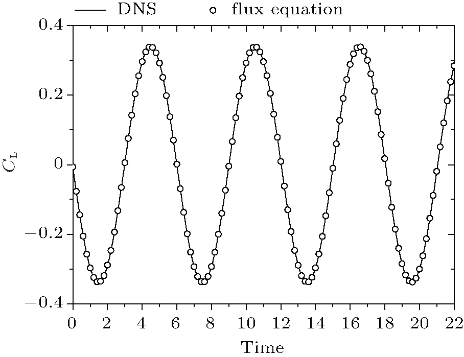 | Fig. 1. Comparison between lift forces evaluated by the Flux equation (the circles) and the DNS results (the solid line). |
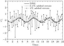
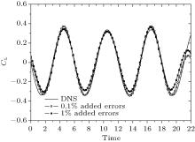
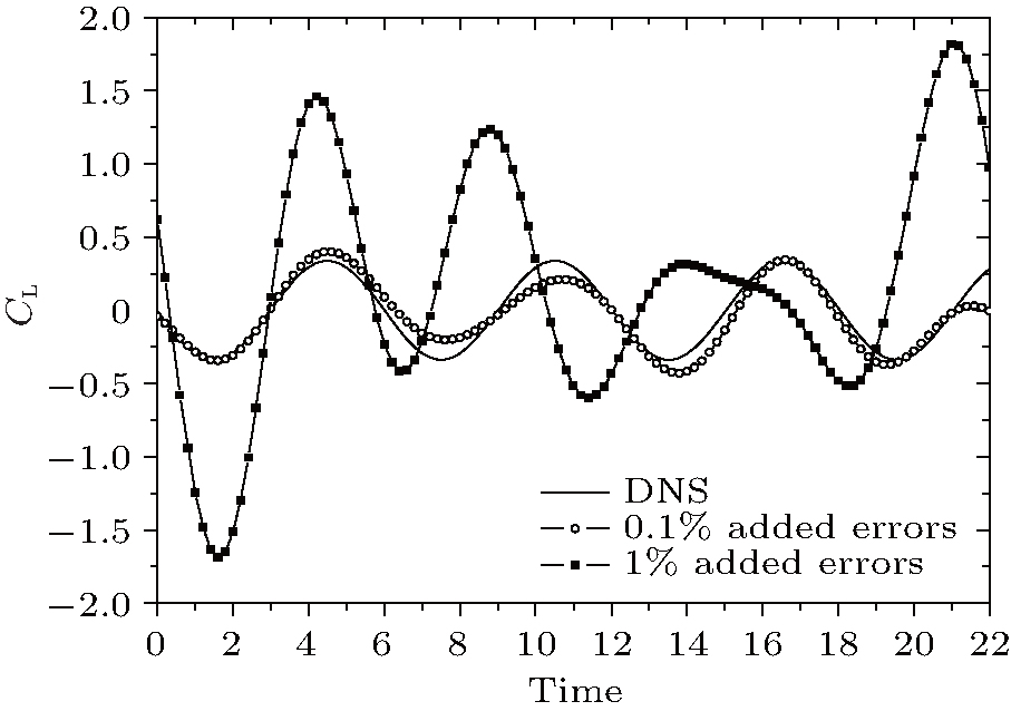
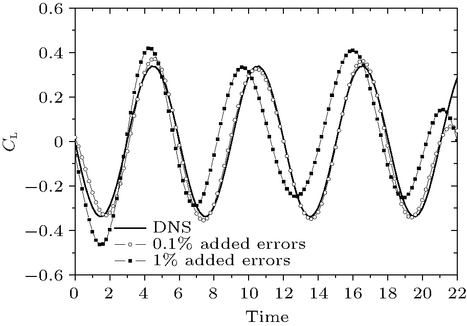
The process of producing the error-added dataset is implemented by MATLAB software. The random numbers are produced by the function “ randn” and “ rand” . The former one produces standard normally distributed random numbers with the mean 0 and the standard deviation 1, while the latter one produces uniformly distributed random numbers in a range of 0– 1. As the uniform velocity is 1, the random numbers on the order of 0.01 (or 0.001) are added in each velocity component as 1% (or 0.1%) experimental errors. We use 0.01 × randn (or 0.001 × randn) to produce standard normally distributed experimental errors on the order of 1% (or 0.1%), while use 0.02 × (rand-0.5) (or 0.002 × (rand-0.5)) to produce uniformly distributed experimental errors on the order of 1% (or 0.1%). The lift forces evaluated by the flux equation from the artificial dataset with the two distributed errors are shown in Figs. 2 and 3 respectively. The results of the artificial dataset with 0.1% error are close to the DNS results, while the result of the artificial dataset with 1% error seems to be submerged by high-frequency noises.
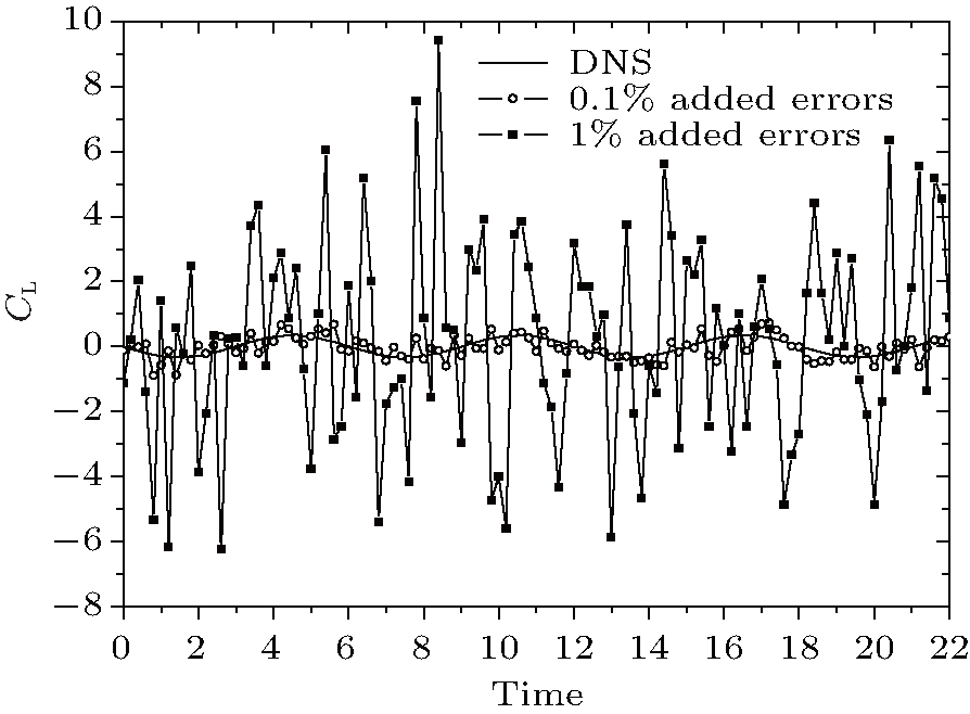 | Fig. 2. Lift forces evaluated by the flux equation from the artificial dataset with standard normally distributed errors on the order of 0.1% and 1% respectively. |
 | Fig. 3. Lift forces evaluated by the flux equation from the artificial dataset with uniformly distributed errors in the order of 0.1% and 1% respectively. |
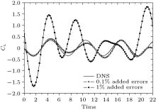
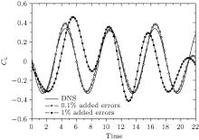
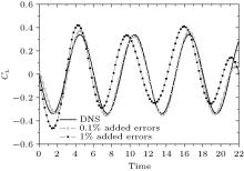
To get rid of the errors in obtained lift forces, the results of Noca’ s method and the novel method are compared with each other. The spectrum of artificial error-added data shows that vortices-shedding frequency is approximately 0.18 Hz which agrees with the experimental result given by Williamson.[20] It is safe to select the frequency which is larger than the vortices-shedding frequency and smaller than the frequency of the next peak in the spectrum as the cutoff frequency. We use 0.25 Hz here, since the results of low-pass filter are very close in a range from 0.19 Hz to 0.3 Hz, which also agrees with Noca’ s experimental results.[11] Figures 4 and 5 show the results from the Noca’ s method. For the artificial data with 0.1% added error, the evaluated lift forces are close to the DNS results. While for the artificial data with 1% added error, the evaluated lift forces are completely different from the DNS results. The Noca’ s method is inapplicable for evaluating the lift forces from the dataset with 1% experimental error, although this error level is acceptable in PIV measurements. To apply the novel method, we choose the square control volumes without any common boundary along the PIV data points. As the result of the novel method is gradually close to the result of DNS with the number of control volumes increasing, and the size of dataset is finite, the results of 21 square control volumes whose diagonal vertices are (2+ n, 2+ n), (199 − n, 199 − n) are shown in Figs. 6 and 7 as an example, where n is the integer number from 1 to 21. The cutoff frequency of the low-pass filter is also 0.25 Hz. It is concluded that the evaluations of the lift forces are significantly improved by the novel method for the dataset with the two distributed errors.
 | Fig. 4. Lift forces evaluated by the Noca’ s method from the artificial dataset with standard normally distributed errors. The cutoff frequency of the low-pass filter is 0.25 Hz. |
 | Fig. 5. Lift forces evaluated by the Noca’ s method from the artificial dataset with uniformly distributed errors. The cutoff frequency of the low-pass filter is 0.25 Hz. |
 | Fig. 6. Lift forces evaluated by the novel method from the artificial dataset with standard normally distributed errors. The cutoff frequency of the low-pass filter is 0.25 Hz. |
 | Fig. 7. Lift forces evaluated by the novel method from the artificial dataset with uniformly distributed errors. The cutoff frequency of the low-pass filter is 0.25 Hz. |
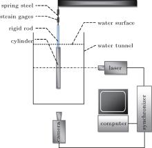
The novel method is also applied to an experimental dataset. The experiment is implemented in a water channel whose test section is 5.4 m × 0.25 m× 0.3 m (length × width × depth) and the free-coming stream velocity ranges from 0.05 m/s to 0.4 m/s. A plexiglass cylinder with a length of 0.15 m is submerged in water. As the free-coming stream velocity is close to 0.09 m/s and the diameter of the cylinder is 0.01 m, the Reynolds number based on them is approximately 900.
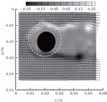
Figure 8 shows the experimental setup which is designed to measure the lift forces by strain gauges and time-resolved particle image velocimetry (TRPIV) simultaneously. The sample rate of strain gauges is 100 Hz, while the sample rate of the TRPIV system is 500 Hz. The 10-μ m glass particles seeded in the flow are illuminated by the laser with single-frame mode, and the results are recorded by 1280× 1024 pixels images. In the post-processing, the interrogation window is set to be 32× 32 pixels, and the window spacing overlapped rate is 75%, therefore, there are 156× 124 vectors in each velocity field. The vectors are recorded as (1, 1) from down left to up right as (156, 124). Figure 9 shows the velocity and vorticity fields. Since the vectors are too dense, it only displays 36× 32 vectors in the velocity field. The velocity and vorticity fields are not well resolved in the region surrounded by the dotted line due to the free end of the cylinder as shown by Noca’ s analysis in his thesis.[11]
 | Fig. 8. Setup of the experiment for flow past cylinder at approximately Re = 900. |
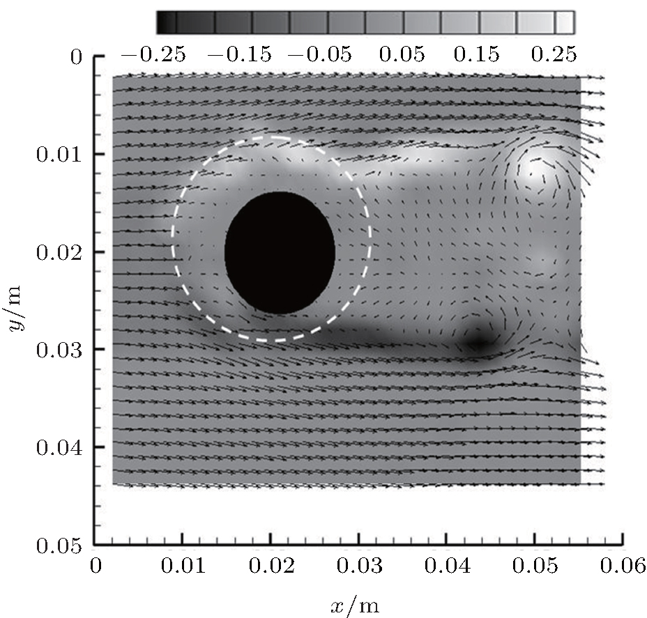 | Fig. 9. Velocity and vorticity field of the experiment. The unresolved region is surrounded by the dashed line. |
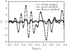
To calculate the lift forces, we use the Noca’ s method and the novel method, and then compare their results with the result of strain gauge. When using the Noca’ s method, we choose the control volumes which avoid the region in the dotted line circle in Fig. 9. As the results of different square control volumes have obvious differences in phase and amplitude between each other, we only show the result of the square whose diagonal vertices are (3, 3), (154, 122) as an example. When using the novel method, we also need to avoid the region in the dotted line circle in Fig. 9, where only the 21 square control volumes whose diagonal vertices are (2 + n, 3), (155 − n, 123 − n) can be used, where n is the integer number from 1 to 21. Although the spectrum of the lift forces obtained by the strain gauge shows that vortices-shedding frequency is approximately 1.74 Hz which agrees with the experimental result given by Roshko, [21] we set 3.2 Hz as cutoff frequency to reserve the natural frequency of the measurement system which is approximately 3.1 Hz. Figure 10 compares the results obtained by using the Noca’ s method and the novel method with the result of strain gauge. It can be observed that the result of the novel method matches well with that of the strain gauge.
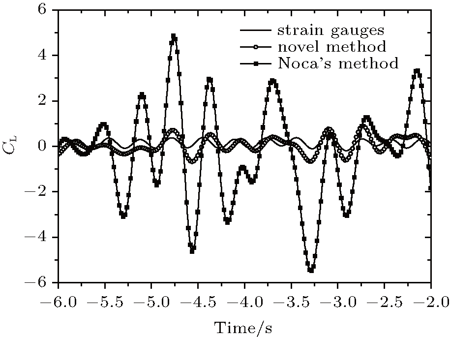 | Fig. 10. Lift forces which are obtained by the strain gauge, the Noca’ s method, and the novel method. The cutoff frequency of the low-pass filter is 3.2 Hz. |
The present study focuses on the effect of experimental errors in PIV measurement on evaluating the lift forces by using Noca’ s flux equation. It verifies that Noca’ s method is inapplicable in the PIV dataset with 1% experimental error even if the effect of numerical errors on evaluating lift forces can be ignored. A novel method which is also based on the flux equation is proposed to solve the problem. As Noca’ s method uses the flux equation in one single control volume in combination with low-pass filter, the new development in this method is that multiple control volumes are used and does not increase more cost. However, the results obtained demonstrate that this method effectively removes the errors which are generated by the experimental errors in PIV measurements. The main conclusions are as follows.
(i) The low-frequency errors in the evaluated lift forces increase with the experimental errors increasing. When the experimental errors are less than 0.1%, the generated low-frequency errors in lift forces can be ignored. When the experimental errors are larger than 1%, the low-frequency errors generated in lift forces are very large so that they must be eliminated.
(ii) Taking the mean lift force from multiple control volumes can minimize low-frequency errors efficiently. But we should note that the control volumes are finite due to the finite size of PIV dataset, so that some low-frequency errors are still left in the results. Therefore, other effective methods are needed to get rid of the low-frequency errors in more complicated situations.
(iii) This paper only considers the random errors as experimental errors. However, other situations that the experimental errors contain large systematic errors or the spatial and time resolutions are not sufficient for differential and integral, need to be further studied. The results are expected to be used for evaluating the lift forces on the MAVs in future.
We would like to thank Dr. Zhu Xiao-Jue for providing us with the original DNS dataset.
| 1 |
|
| 2 |
|
| 3 |
|
| 4 |
|
| 5 |
|
| 6 |
|
| 7 |
|
| 8 |
|
| 9 |
|
| 10 |
|
| 11 | [Cited within:4] |
| 12 |
|
| 13 |
|
| 14 |
|
| 15 |
|
| 16 |
|
| 17 |
|
| 18 |
|
| 19 |
|
| 20 |
|
| 21 |
|