


Direct numerical simulation of viscoelastic-fluid-based nanofluid turbulent channel flow with heat transfer
[Yang Juan-Chenga), b) , Li Feng-Chen†a)  , Cai Wei-Hua
a) , Zhang Hong-Naa) , Yu Boc) ]
, Cai Wei-Hua|
|


†Corresponding author. E-mail: lifch@hit.edu.cn
*Project supported by the National Natural Science Foundation of China (Grant No. 51276046), the Specialized Research Fund for the Doctoral Program of Higher Education of China (Grant No. 20112302110020), the China Postdoctoral Science Foundation (Grant No. 2014M561037), and the President Fund of University of Chinese Academy of Sciences, China (Grant No. Y3510213N00).
Our previous experimental studies have confirmed that viscoelastic-fluid-based nanofluid (VFBN) prepared by suspending nanoparticles in a viscoelastic base fluid (VBF, behaves drag reduction at turbulent flow state) can reduce turbulent flow resistance as compared with water and enhance heat transfer as compared with VBF. Direct numerical simulation (DNS) is performed in this study to explore the mechanisms of heat transfer enhancement (HTE) and flow drag reduction (DR) for the VFBN turbulent flow. The Giesekus model is used as the constitutive equation for VFBN. Our previously proposed thermal dispersion model is adopted to take into account the thermal dispersion effects of nanoparticles in the VFBN turbulent flow. The DNS results show similar behaviors for flow resistance and heat transfer to those obtained in our previous experiments. Detailed analyses are conducted for the turbulent velocity, temperature, and conformation fields obtained by DNSs for different fluid cases, and for the friction factor with viscous, turbulent, and elastic contributions and heat transfer rate with conductive, turbulent and thermal dispersion contributions of nanoparticles, respectively. The mechanisms of HTE and DR of VFBN turbulent flows are then discussed. Based on analogy theory, the ratios of Chilton–Colburn factor to friction factor for different fluid flow cases are investigated, which from another aspect show the significant enhancement in heat transfer performance for some cases of water-based nanofluid and VFBN turbulent flows.
Heat transfer performance and flow resistance are the two key factors to be considered in determining whether a fluid is suitable for an engineering application. In the past decades, a variety of techniques have been utilized to improve heat transfer rate in order to reach a high thermal efficiency and/or reduce flow resistance in order to obtain low power consumption of pump, which leads to energy-saving effect finally. Heat transfer rate can be enhanced by modifying the structure of heat transfer surface passively or enhancing thermal properties (e.g., thermal conductivity) of the working fluid. Similarly, flow resistance can also be reduced by modifying flow geometry and boundary conditions or changing fluid properties such as through adding drag-reducing polymer or surfactant additives in turbulent flow state.
Within the methods for heat transfer enhancement (HTE), the increasing of fluid thermal conductivity by the addition of nanoparticles into conventional liquid is a hot research topic because of its significant effectiveness in enhancing convective heat transfer rate with only minor effort. Choi et al. did pioneering work on studying the thermal conductivity of the nanoparticle-laden liquid and referred to this kind of fluid as nanofluid. In his research, 160% enhancement in thermal conductivity of engine oil with 1%-volume carbon nanotubes added was obtained.[1] By suspending nano-sized copper particles in ethylene glycol, Eastman et al.[2] obtained 40% enhancement in thermal conductivity. Many other research groups[3− 5] also obtained thermal conductivity enhancement of nanofluid by utilizing different kinds of nanoparticles such as TiO2, Al2O3, CuO, Ag, etc. Due to the increased thermal conductivity of nanofluid as compared with its base fluid, enhancement in heat transfer is the superior characteristic of nanofluid flows.[6, 7] Xuan and Li, [8] and Li and Xuan[9] experimentally studied the flow and heat transfer features of water-based copper nanofluid in a horizontal pipe at laminar and turbulent flow states, respectively. Their results showed that the heat transfer rates of copper nanofluid flows increased remarkably compared with that of water flow at the same Reynolds numbers, while the pressure drops had no significant increase. Ding et al.[10] carried out experimental studies on convective heat transfer of carbon nanotube (CNT) nanofluid flows, and observed up to 350% enhancement in heat transfer rate. Utilizing TiO2 as nanoparticles, Sajadi and Kazemi[11] investigated flow and heat transfer characteristics of TiO2 nanofluid, and obtained obviously a higher flow resistance for nanofluid than that of the base fluid, which was contradicted to the results given by Xuan and Li.[8]
From the viewpoint of numerical simulations, single-phase method and two-phase method are the two typical approaches to simulating nanofluid flows. The single-phase method assumes that the suspended solid particles are in thermal equilibrium with the fluid phase and no relative velocity exists between solid and fluid phases, implying that the particles move at the same velocity as the base fluid elements.[12] Some numerical simulations were performed for nanofluid flows based on the single-phase model, [13, 14] from which acceptable results were obtained for heat transfer and hydrodynamic characteristics of nanofluid flows as compared with experimental data. Since the single-phase method for nanofluid flows only adopts the changed thermophysical properties of fluid in the momentum and energy equations of nanofluid flow, it is thus improper to be used for exploring the mechanism of HTE. The two-phase model, which can describe the slip velocity and interaction between fluid and nanoparticles, is also developed to simulate heat transfer performance of nanofluid flows. By using this model, Mirmasoumi and Behzadmehr, [15] and Kalteh et al.[16] simulated a water-based Cu nanofluid flow and obtained more precise heat transfer results than by using the single-phase model. However, compared with single-phase model, the two-phase model consumes more computer resources because the coupled equations should be numerically solved simultaneously. In order to obtain a balance between computer resource consumption and precision of results, some modifications on the single-phase model were performed for numerical simulation of nanofluid flows. Xuan and Li, [12] and Xuan and Roetzel[17] introduced a thermal dispersion model to explain the mechanism of HTE resulting from chaotic movement of nanoparticles in the main flow, and proposed a theoretical correlation for heat transfer of nanofluid flow based on this model. Heris et al., [18] Ö zerincc et al., [19] Mokmeli and Saffar-Avval, [20] and Khanafer et al.[21] inherited and developed a thermal dispersion model and utilized this model to investigate the characteristics of laminar flow and heat transfer of nanofluids. It showed that numerical simulation results by means of the thermal dispersion model are in good agreement with experimental data. However, the thermal dispersion model has been used only to simulate nanofluid flows at laminar state so far, and so some modifications should be made before its application to turbulent flows of nanofluid. Very recently, referring to the ideas reported in previous studies, the present authors proposed a new thermal dispersion model particularly for turbulent flow of nanofluid, which has been successfully used to simulate the nanofluid flow and heat transfer at turbulent state.[22]
Within the approaches to realizing flow DR, the addition of viscoelastic drag-reducing additives such as long-chain polymer or some surfactants is the most effective technique with great potential. The turbulent DR phenomenon by drag-reducing additives was first reported by Toms in 1948.[23] The aqueous solution of drag-reducing polymer or surfactant additives is normally a viscoelastic fluid, and the viscoelasticity interacts with turbulence so as to significantly reduce the flow resistance at turbulent flow state. Experimental results showed that turbulent DR rate can even reach 80% at a dilute mass concentration of polymer.[24] Luchik and Tiederman[25] adopted laser Doppler velocimetry (LDV) to study the DR effect of aqueous polymer solution channel turbulent flow. Their experimental results revealed that the reduction of velocity fluctuation intensity in the flow direction and the decrease of energy transportation from the flow direction to the wall-normal direction were the main reason of DR. Zakin et al.[26] experimentally studied the DR phenomenon in an aqueous surfactant solution turbulent flow, focusing on velocity distribution in flow region, rheology characteristic, the molecular structure effects, and counterions effects on DR, and finally obtained the asymptote of the friction factor for surfactant drag reducer solution turbulent flow. Li et al.[27] utilized particle image velocimetry (PIV) to measure the flow characteristics of surfactant solution turbulent flow in a two-dimensional (2D) channel, and their results showed that compared with the scenario in water flows, the mean flow velocity in the near-wall region, velocity gradient in the wall-normal direction near the wall, and the wall shear stress decreased in the surfactant solution flows, which resulted in a drag-reducing effect. Li et al.[28, 29] also simultaneously measured the fluctuating velocity and temperature fields by using LDV combining with a home-made fine-wire thermocouple probe in a dilute aqueous surfactant solution flows in a horizontal 2D channel. It was obtained that turbulent DR was always accompanied with convective heat transfer deterioration, and the heat transfer reduction (HTR) rate was larger than the turbulent DR rate. The occurrence of HTR is due to the significant suppression of velocity fluctuation intensity in the wall-normal direction, which results in a great decrease of energy transport as well as momentum transport between the turbulent flow field and solid boundary.[29]
Many studies on turbulent drag-reduced flows by additives have also been reported so far by numerical simulations, most of which were direct numerical simulations (DNS) method, some of which adopted Reynolds averaged Navier– Stokes (RANS) model and very few of which adopted large eddy simulations (LES) technique. Some examples of numerical simulations of turbulent drag-reducing flows are reviewed as follows. Cai et al.[30− 32] and Li et al.[33] performed the numerical studies of the characteristics of DR in homogeneous isotropic turbulence with polymer additives, focusing on how the fluid viscoelasticity influences the turbulence structures, turbulent kinetic energy cascading procedure, turbulence scaling law, etc. Yu et al.[34] and Tsukahara[35] reported the DNS studies of turbulent drag reducing flows of viscoelastic fluid in a 2D channel by using the Giesekus model as the constitutive equation for the viscoelastic fluid. They focused on investigating the effects of model parameter on DR, developing efficient finite difference methods, exploring the mechanism of DR and HTR, etc. However, although DNS method can resolve detailed flow field up to the smallest scale of turbulence, it needs huge computation consumptions especially in large Reynolds number condition. The RANS method can meet the needs for engineering flow problems, which usually have large Reynolds numbers. Pinho et al., [36] Resende et al., [37] and Leighton et al.[38] established some preliminary Reynolds stress models based on FENE-P constitutive equation for turbulent drag reducing flows. Some predicted variables such as mean velocity, strain, etc., but not all variables in their computation field, were in good agreement with DNS data. As for LES of turbulent drag-reducing flow by additives, only a few papers were published, such as those by Thais et al.[39] and Wang et al.[40]
From the above-mentioned overviews, we learn that nanofluid behaves as convective HTE ability and viscoelastic fluid has turbulent DR feature. Then, it is natural to raise a question: how about the combination of the two effects steaming from the two kinds of fluids respectively? It can be conjectured that adding nanoparticles into viscoelastic fluid may form a new fluid, which behaves as turbulent DR characteristics (the comparing target can be the Newtonian-base fluid of normal nanofluids) and HTE (the comparing target can be the turbulent drag-reducing viscoelastic base fluid) as well. The answer to this question is positive. Some preliminary experimental results of this kind of fluid have been published. Liu and Liao, [41] and Liao and Liu[42] added CNTs into viscoelastic aqueous solution of cetyltrimethyl ammonium chloride (CTAC), and referred to this mixture as drag-reducing nanofluid. Their experimental results indicated that there was no obvious difference in drag-reducing characteristic but there appeared obvious differences in heat transfer characteristic between conventional drag-reducing fluid and drag-reducing nanofluid. That is, an enhancement of heat transfer was obtained from drag-reducing nanofluid flow. Yang et al.[43– 46] successfully prepared a new nanofluid with dispersion of copper (Cu) nanoparticles in the viscoelastic aqueous solution of CTAC and sodium salicylate (NaSal), and referred to this kind of nanofluid as viscoelastic-fluid-based nanofluid (VFBN). Detailed experimental studies on thermophysical and rheological properties of the prepared VFBNs, and the characteristics of convective heat transfer and flow resistance in VFBN turbulent flows have been carried out. The results showed that VFBN turbulent flows behave as obvious DR (compared with water flow) and relative convective HTE (compared with the viscoelastic base fluid flow). Nevertheless, only some overall information such as heat transfer coefficient and pressure drop in the flow could be obtained in experiment. It is obviously not enough to understand in depth the mechanisms of turbulent DR and HTE of VFBN. The mechanism study calls for DNS. To the author’ s best knowledge, no DNS studies have been carried out so far for a VFBN turbulent flow. Actually, DNS studies on turbulent flows of a conventional nanofluid are also scarce.[47– 49]
In the present study, we perform DNSs of VFBN turbulent flows with heat transfer and aim at exploring the mechanisms of DR and HTE induced by VFBN. The DNS of VFBN turbulent flow is implemented by combining with our previous efforts including Yu and Kawaguchi’ s, [34] which presented the method of DNS study of drag-reducing turbulent flow of viscoelastic fluid, and Yang et al.’ s[22] which presented the method of DNS study of the convective heat transfer of nanofluid turbulent flow. Based on DNS database, the influences of viscoelasticity, volume fraction of nanoparticles, and flow Reynolds number on the performance of VFBN turbulent flows are studied. Finally, the mechanisms of DR and HTE of VFBN turbulent flows are investigated.
An overview of the thermal dispersion model proposed for turbulent flows of nanofluids is given below.[22] At first, the energy equation for nanofluid flow considering thermal dispersion effect is written as[18– 22]
where T is the temperature, uj is the velocity, ρ n is the density of nanofluid, kn is the thermal conductivity of nanofluid, t is the computation time, xj is the coordinate, Cp, n is the specific heat of nanofluid, and Kd, j is the dispersion thermal conductivity.
The dispersion thermal conductivity Kd, j takes into account the thermal dispersion effects of nanoparticles, which introduces an additional term into the normal energy equation for a single-phase fluid flow. The proposed Kd, j model for turbulent flow of nanofluids considers the influences of volume fraction of nanoparticles, size of nanoparticle, characteristic length scale of turbulent flow, and dimensional consistency, and is expressed as follows:[22]

where C is the constant thermal dispersion coefficient, dp is the diameter of nanoparticle, L is the characteristic length of flow, and φ is the volume fraction of nanoparticles.
For the details of the proposed thermal dispersion model Eq. (2), one refers to Ref. [22]. Substituting Eq. (2) into Eq. (1), the energy equation considering nanofluid thermal dispersion effect at turbulent flow state becomes,
By directly solving Eq. (3), the instantaneous temperature field of VFBN fluid turbulent flow can be obtained. Note that an important factor influencing the DNS results of convective heat transfer in nanofluid turbulent flow is the value of the constant thermal dispersion coefficient C. This value can be determined by experimental data. In our previous study of the thermal dispersion model for copper nanofluid turbulent flow, [22]C = 1.23 × 10− 7 is obtained through comparing DNS result with experimental data. In the present simulation, C = 1.23 × 10− 7 is also utilized.
The 2D channel and pipe are the two typical geometrical models used in the DNS study of a wall-bounded turbulent flow with heat transfer. In the present study, the channel flow geometry is adopted for our DNSs of VFBN turbulent flow, which is schematically shown in Fig. 1. As plotted in Fig. 1, x, y, and z represent the streamwise, wall-normal, and spanwise directions, respectively. The channel height is 2h. The periodic boundary condition is used in the flow and spanwise directions, respectively. The periodic length of the computation domain is determined by the flow state. In the flow direction, the length should be larger than the characteristic length of the largest scale of turbulent coherent structure. The length of turbulent flow structure near the channel wall in the streamwise direction is about 1000/Reτ h, where Reτ is the Reynolds number determined by the friction velocity 
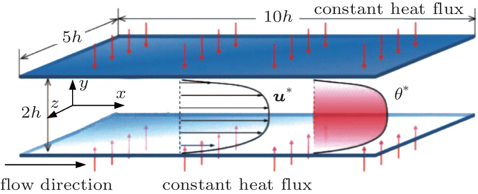 | Fig. 1. Geometrical model of computation domain. |
Use the following non-dimensional parameters: non-dimensional length 


(here, the prime ′ and the bar ̅ mean the fluctuation and mean part of variables), non-dimensional conformation 
Continuity equation

Momentum equation

where

is the Kronecker delta, Reτ = ρ buτ h/(μ b + η b), and 
Giesekus constitutive equation for conformation field
Energy equation
where Pr = ρ bCp, b (μ b + η b)/kb is Prandtl number, 
For DNS of a wall-bounded turbulent flow, the near-wall grid quality is of critical importance because the vortex with the smallest length scale near the solid wall boundary needs to be resolved. Thus, the near-wall grid density is increased using the following equation

where k is the identifier of the k-th grid in the y direction, N is the total grid number in the y direction, a is a parameter for adjusting the variation of gird density near the wall, and ς k is factor of grid size.
Staggered grid system is used to avoid a zigzag pressure field in the computation field. The pressure, temperature, and conformation components are stored in the cell center while velocity components are stored at the cell borders. The non-slip boundary is used on both channel walls. The flow is heated with a uniform heat flux from both walls of channel. Initial instantaneous turbulent velocity and temperature fields, [50] which accord with statistical characteristics of wall-bounded turbulence, are used to obtain a fully developed turbulent flow state when the calculation is converged.
In the spatial discretization process of momentum equation and energy equation, the second-order central difference scheme is used to discretize the convection term and diffusion term. In the time discretization process of momentum equation, the fractional step method using the Adams– Bashforth scheme for the time advancement is adopted. Because the constitutive equation has a very strong nonlinear property, the MINMOD scheme is utilized to discretize the convective term to guarantee calculation stability.[34] And other terms of the constitutive equation are discretized with the second-order central difference scheme. Multi-grid method is used to accelerate the convergence of calculation.
Table 1 shows the simulation cases in the present study. Copper particles with an average diameter of 60 nm are used as the nanoparticles. For viscoelastic base fluid, α is set to be 0.001. The time step is set to be 3 × 10− 4 for Newtonian fluid cases (water and water-based nanofluid), and 1 × 10− 4 for non-Newtonian fluid cases (viscoelastic base fluid and VFBN). For each case, in order to obtain a more creditable result, 200 frames of data are collected after the flow and heat transfer have been under statistically fully developed conditions. In Table 1, BF represents the water-base fluid case; VBF represents the viscoelastic-base fluid case; NF represents the water-based nanofluid case; VFBN represents the viscoelastic-fluid-based nanofluid case. For the simulation of nanofluid turbulent flow, the influences of Reynolds numbers (NF3-N, NF4-N, NF5-N, VFBN3-N, VFBN4-N, VFBN5-N) and volume fractions of nanoparticles (NF1-N, NF2-N, NF3-N, FBN1-N, VFBN2-N, VFBN3-N) are considered in the following elucidations and discussion.
| Table 1. Simulation cases and corresponding settings in the present DNSs. |
For a wall-bounded turbulent flow, the solid wall plays an important role in inducing and evolving turbulent vortices. To capture full flow information, the grid size near the wall must be fine enough to resolve vortex structures at the Kolmogorov scale theoretically. However, for a certain computation region, smaller grid size means larger grid number and greater computation loads. Thus, in order to check the influence of grid density on the simulation results, three grid systems for the simulated channel flow are tested. The grid numbers in the y direction (wall-normal direction) are set to be 64, 128, and 256, respectively. The grid numbers in the x and z directions are set to be constant (Nx = Nz = 64) because periodic boundary condition is adopted in these directions. The typical Newtonian fluid turbulent flows with heat transfer at Pr = 5.0, Reτ = 180, and 395, respectively, are used to verify the accuracies of the present simulations. Figures 2– 5 show the simulation results as compared with the results of Kawamura et al.[51] under the same conditions and the results calculated by theoretical or empirical formula.
For a Newtonian fluid turbulent flow, the non-dimensional velocity satisfies linear distribution in the viscous sublayer:

and log-law distribution in the log-law layer:[52]

For convective heat transfer in a Newtonian fluid flow, the non-dimensional temperature difference conforms to linear distribution in the viscous sublayer:

and the thermal boundary log-law distribution in the log-law layer (Pr < 6.0)[52]

where y+ = y* Reτ .
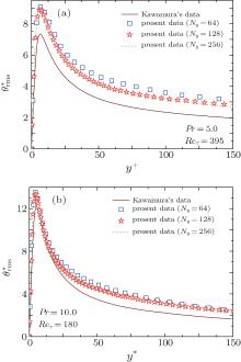
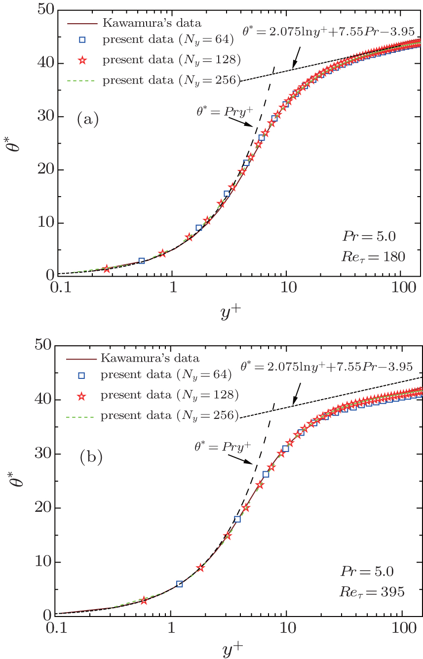 | Fig. 2. Comparisons of mean temperature difference between the present DNS data and previous data:[51] (a) Pr = 5.0, Reτ = 180 and (b) Pr = 5.0, Reτ = 395. |
Figures 2 and 3 show that the distributions of mean temperature and mean streamwise velocity have no obvious differences for the three tested gird systems. Our DNS data show excellent agreement with Kawamura’ s data[51] for the temperature distribution, but they are slightly lower than Kawamura’ s data for the velocity distribution at y+ > 10 (in the main flow region). Compared with the results from the theoretical formula, our DNS results of the mean data of temperature and velocity also show good agreement with those from Eqs. (9) and (11) in the viscous sublayer. In the main flow region, the distribution of mean streamwise velocity is well consistent with Eq. (10), while the distribution of mean temperature difference has some differences from that obtained from Eq. (12), and also from the Kawamura’ s data.[51]
 | Fig. 3. Comparisons of mean streamwise velocity between the present DNS data and previous data.[51] (a) Pr = 5.0, Reτ = 180 and (b) Pr = 5.0, Reτ = 395. |
Figures 4 and 5 show the root-mean-squares (RMSs) of temperature difference (fluctuation intensity) and the streamwise velocity component for the three tested grid systems. From Fig. 4, we can see that the difference between fluctuation intensities of temperature difference decreases when the grid number in the y direction is increased from Ny = 64 to Ny = 128. Nonetheless, there are no visible differences between those of Ny = 128 and Ny = 256. The present DNS result is slightly larger than Kawamura’ s data, especially for the case at larger Reynolds number (Reτ = 395). For the fluctuation intensity of the streamwise velocity (Fig. 5), there are no visible differences when the tested gird number in the y direction is increased.
 | Fig. 4. Comparisons of temperature difference fluctuation result between the present DNS data and previous data:[51] (a) Pr = 5.0, Reτ = 395 and (b) Pr = 10.0, Reτ = 180. |
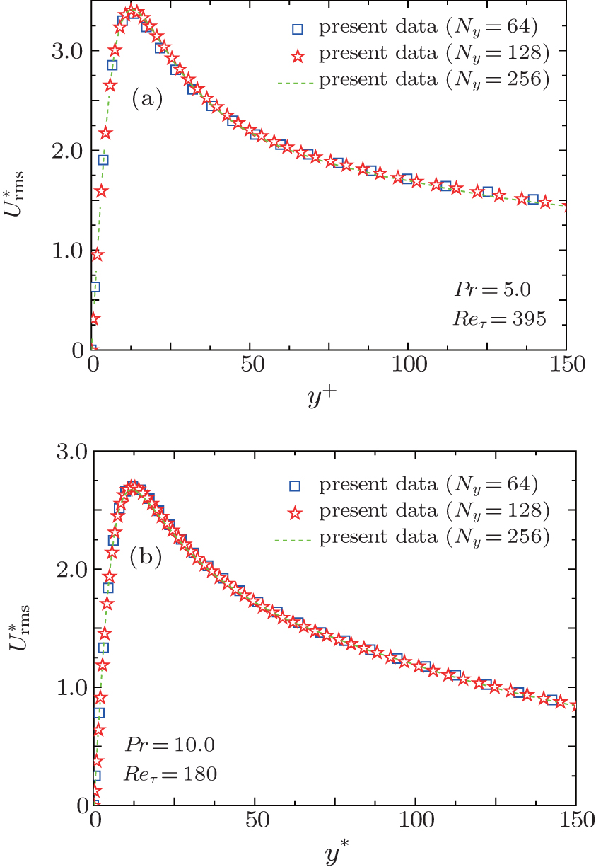 | Fig. 5. Comparisons of velocity fluctuation result among the three tested grid systems: (a) Pr = 5.0, Reτ = 395 and (b) Pr = 10.0, Reτ = 180. |
Our grid verification results are also consistent with those given by Yu et al.[53] when the grid number in the y direction is increased from 64 to 96 in their simulations. According to the above grid verification results of temperature difference and velocity, we can make sure that the present DNS results have no visible difference when the grid number in the y direction is not less than 128. Consequently, in the following discussed DNS cases, and the grid number is set to be 64 in the x, z directions and 128 in the y direction.
The analysis of mean features of turbulent velocity and temperature fields is a direct way to understand the characteristics of flow resistance and heat transfer. Some mean features of the simulated VFBN turbulent flow are elucidated in this section.
Figure 6 shows the mean velocity distributions of BF, VBF, and VFBN flows at Reτ = 180. As shown in Fig. 6(a), the velocity distributions of BF flow are the same as those of VBF flows at y+ < 5, but quite different after y+ > 5. For the VBF turbulent flow, the buffer layer near the wall is thicker than that in the BF flow, while the velocity level in the buffer layer is larger than that in the BF flow. Virk et al.[54] proposed an empirical equation (Eq. (13)) to show the velocity distribution at the asymptotic DR rate. From Fig. 6(a), we can see that the velocity predicted by Eq. (13) agrees well with the present DNS results in the buffer layer, but is larger than DNS results after y+ > 20, which means the simulated cases for VBF flow cannot reach the maximum DR rate. This trend is also consistent well with our previous experimental studies on the drag-reducing turbulent flows by additives[44]

As for VFBN flow (Fig. 6(b)), the mean velocity in the main flow region is lower than that for the VBF flow at the same Reynolds number, but still higher than that of water flow (as compared with Fig. 6(a)).
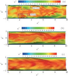
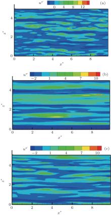
Figure 7 shows the Reynolds-decomposed (fluctuating) velocity vector distributions together with the contour maps of the instantaneous streamwise velocity component in the x– y plane for three different fluid cases (Newtonian fluid, viscoelastic fluid, and VFBN), demonstrating the characteristics of turbulent bursting events and coherent structures in the different fluid flows. Figure 7(a) displays the results of BF fluid (water) flow, from which obvious turbulent bursting events, i.e., ejection of low-momentum fluid from the wall and sweep of high-momentum fluid toward the wall (as marked in the figure as examples), can be observed. However, the turbulent bursting events are significantly depressed at its frequency for both the VBF and VFBN flows, as indicated in Figs. 7(b) and 7(c), respectively. The depression of turbulent bursting events results in the occurrence of turbulent DR as shown later.
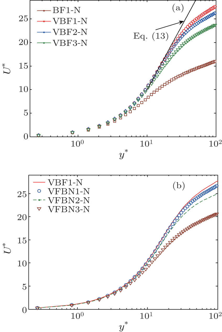 | Fig. 6. Mean velocity profiles for different fluid flows at Reτ = 180. Comparisons (a) between BF and VBF cases and (b) between VBF and VFBN cases. |
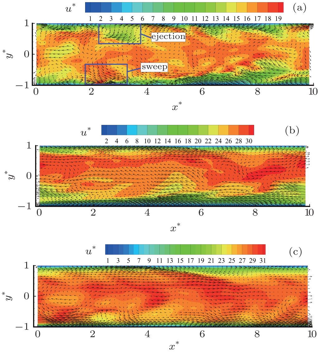 | Fig. 7. Instantaneous velocity fields in the x– y plane for three typical fluid flows (Reτ = 180). (a) BF1-N case, (b) VBF1-N case, and (c) VFBN1-N case. |
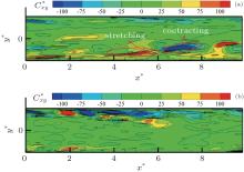
In order to obtain insightful information about the microstructures in the VBF and VFBN flows, which should be closely related to the depression of turbulent bursting events, the conformation fields in these two typical fluid flows are shown in Fig. 8. It can be clearly seen from the conformation contour map that the microstructures are stretched or contracted near the wall. The microstructures existing in viscoelastic fluid behave as elastic strings, which can store turbulent energy when stretched and release energy when relaxed. These changes of microstructures induced by the large velocity gradient can reduce the velocity gradient in return, and finally depress the occurrence of turbulent bursting events. Our simulation results are consistent with other’ s research results on the interaction between microstructures of polymer or surfactant and velocity field.[31, 33]
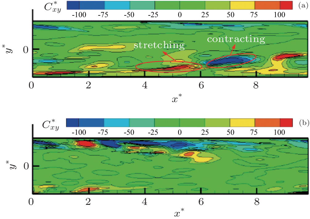 | Fig. 8. Conformation fields of two typical viscoelastic fluid flows in the x– y plane (Reτ = 180). (a) VBF1-N case, and (b) VFBN1-N case. |
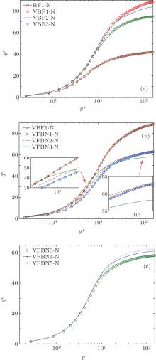
Figure 9 shows the profiles of mean temperature difference of BF, VBF, and VFBN flows at different values of Weissenberg number (We), volume fractions of nanoparticles, and Reynolds numbers. As seen from Fig. 9(a) for the comparison between the BF and VBF cases, the temperature difference of VBF flow is larger than that of BF flow. Moreover, with the increase of We, the temperature difference is increased. The Nusselt number (Nu) can be calculated with Eq. (14). From Eq. (14), we can see that higher temperature difference corresponds to lower Nu or worse heat transfer rate. Consequently, the occurrence of HTR in VBF turbulent flow is revealed from Fig. 9(a). As expected, the temperature difference in VFBN turbulent flow is reduced in the main flow region at the same Reynolds number as compared with the VBF case, which means that the HTE effect is induced by the addition of nanoparticles to the viscoelastic fluid (Fig. 9(b)). The variation of temperature difference in VFBN flows with volume fraction of nanoparticles has no obvious tendency. Thus, we cannot reach a solid conclusion on how the nanoparticle volume fraction influences the HTE only from the temperature difference results.
Figure 9(c) displays the influences of the Reynolds number on the temperature difference of VFBN flows, showing that the temperature difference is reduced (Nu is increased) with the increase of the Reynolds number. The Nu is given as

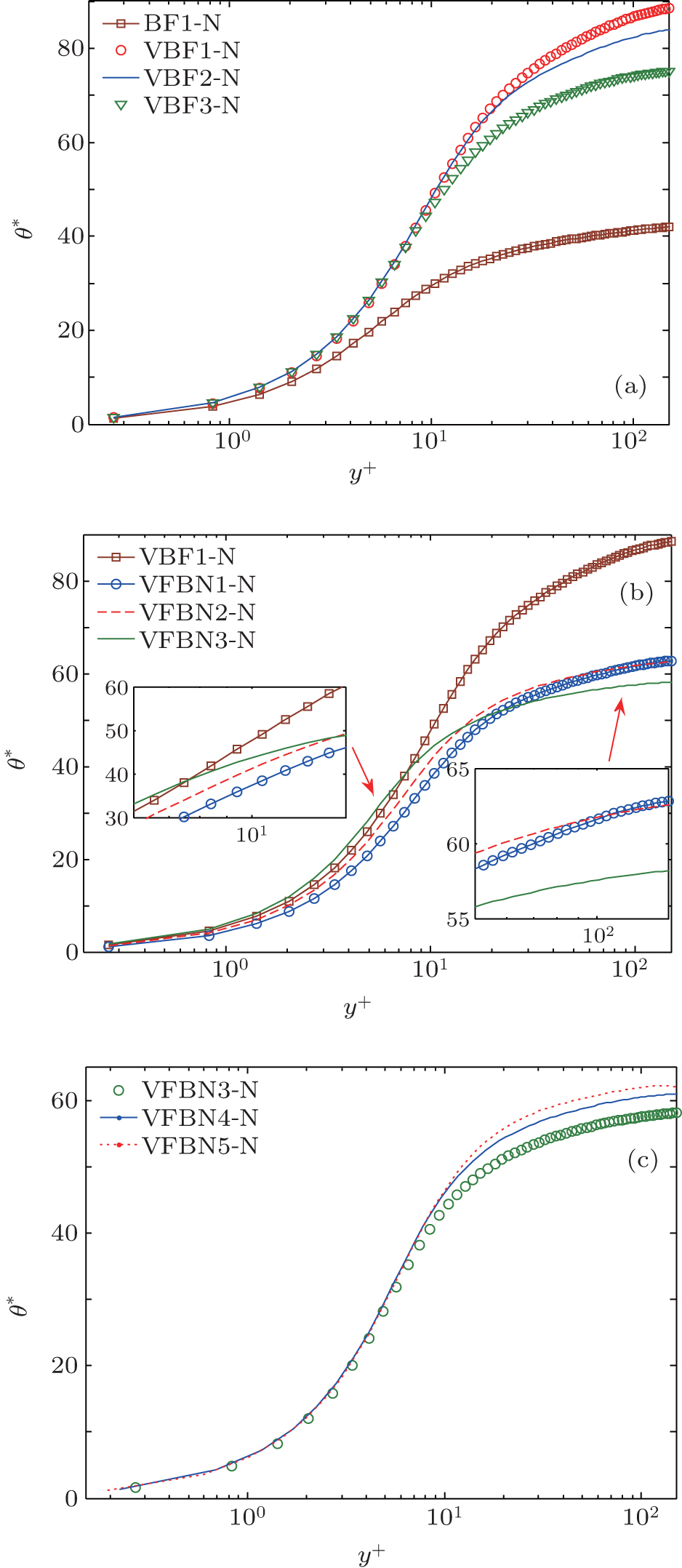 | Fig. 9. Variations of mean temperature difference with y+ for different fluid flows. (a) VBF flows with different We numbers (Reτ = 180), (b) VFBN flows with different volume fractions of nanoparticles (Reτ = 180), and (c) VFBN flows with different Reτ values. |
From the above-mentioned discussion, we know that the viscoelastic fluid flow increases its velocity and temperature profiles as compared with the Newtonian fluid flow at the same Reynolds number, which are linked with turbulent DR and HTR phenomena, respectively. The addition of nanoparticles in VBF improves heat transfer performance but increases flow resistance as well. The definitions of HTE and DR are as follows:


where Cfw is the fanning coefficient of resistance of base fluid, and Cfn is the fanning coefficient of resistance of nanofluid.
In order to evaluate the overall performances of VFBN turbulent flows, a phase diagram categorizing HTEs and DRs for all the simulated cases is shown in Fig. 10. Since the physical significance of this phase diagram (Fig. 10) was stated in detail in our previous experimental study when showing the overall performances of VFBN turbulent flows with heat transfer, [44] it will not be repeated herein.
 | Fig. 10. Phase diagram of HTE versus DR for all the simulated cases. |
Through plotting HTE and DR for all the simulated cases in Fig. 10, the following results can be summarized. The overall performances of VBF (normal viscoelastic fluid) flows are categorized in phase 4 (DR > 0, HTE < 0 with |HTE > |DR|), which means that DR is accompanied with HTR and HTR rate is larger than DR rate. This phenomenon is in good agreement with the previous experimental and DNS studies of normal viscoelastic fluid turbulent flows.[28, 29] The overall performances of NF (normal nanofluid) flows are located on the x axis in the positive direction, which means HTE without increased flow resistance (since nanoparticle effect on the flow is not considered in the present DNSs). The overall performances of VFBN flows are categorized in phase 3 (DR > 0, HTE < 0, |DR| > |HTE), which means that the DR is accompanied with HTR, but HTR rate is smaller than DR rate. HTR rate being smaller than DR rate, which is opposite to the consensus findings for turbulent drag-reducing flows of normal viscoelastic fluids, indicates the characteristic of a relative HTE as compared with the normal viscoelastic fluid turbulent flow cases. The simulated results for the NF, VBF, and VFBN cases in the present study have captured the main characteristics found in our previous experiments, [44] indicating that the presently established DNS method is reliable on one aspect.
In the previous section, the overall characteristics of the simulated flows of different fluids are discussed through presenting the mean velocities, mean temperature differences, HTE, and DR. In this section, some fluctuation characteristics are also analyzed in order to gain an insight into the mechanisms of DR and relative HTE of VFBN turbulent flow.
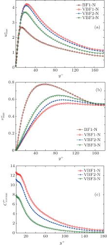
Figure 11 shows root mean square (RMS) profiles of fluctuating velocity components in the streamwise and wall-normal directions (

It can be seen from Fig. 11(a) that the profile of
Figure 11(b) shows that 
 | Fig. 11. Profiles of fluctuation intensities of the streamwise and wall-normal velocity components and a typical component of the conformation tensor for viscoelastic fluid (Reτ = 180). (a) RMS of u, (b) RMS of v, and (c) RMS of Cxx. |
As for the VFBN flows, the profiles of the abovementioned three fluctuation intensities are quantitatively different from those of the VBF flows. Figure 12 shows the results for VFBN flows with different volume fraction of nanoparticles at Reτ = 180. It can be seen from this figure that
 | Fig. 12. Profiles of fluctuation intensities of the streamwise and wall-normal velocity components and a typical component of the conformation tensor for VFBN flows at different volume fractions of nanoparticles (Reτ = 180). (a) RMS of u, (b) RMS of v, and (c) RMS of Cxx. |
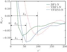
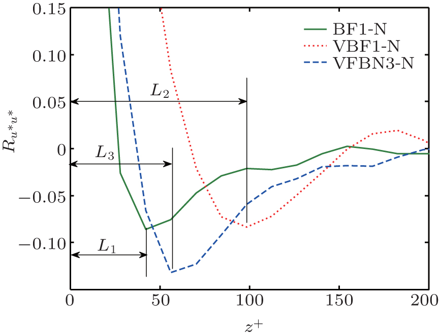
The near-wall low-speed streaks are one of the typical flow structures in the wall-bounded turbulent flow, which reflect the slices of horseshoe vortex legs near the wall. Figure 13 shows the low-speed streak images in the x– z plane taken at y+ = 4.1 for the cases of three typical fluids (BF, VBF, and VFBN). It can be seen that the distribution of the low-speed streaks for the VBF case becomes more regular than for the BF case. For the case of VFBN, the distribution pattern of the low-speed streaks is in between the cases of BF and VBF. Furthermore, in order to obtain some quantitative information about the near-wall low-speed streaks, the spanwise intervals between streaks for the three typical cases are calculated by using the auto-correlation method, which are shown in Fig. 14 for the results. Note that in order to magnify the appearance around the first wave trough in the profile of auto-correlation coefficient Ruu in the spanwise direction, only part of z+ range is plotted in Fig. 14. In this figure, L1, L2, and L3 represent the average spanwise intervals of the low-speed streak for the BF, VBF, and VFBN cases, respectively. At the same Reynolds number, the wider near-wall low-speed streaks corresponds to the lower frequency of turbulent bursting event or the occurrence of coherent structure, which results in lower flow resistance. The present results show that L2 > L3 > L1, which means that the flow resistance of the VFBN flow is larger than that of the VBF flow but lower than that of the BF flow. In other words, the VFBN flow also exhibits the ability to reduce the turbulent drag as compared with the Newtonian fluid,
 | Fig. 13. Instantaneous distributions of the near-wall low-speed streaks for three typical cases in the x– z plane at y+ = 4.1. (a) BF1-N, (b) VBF1-N, and (c) VFBN3-N. |
but the ability to reduce the turbulent drag for VFBN becomes weakened as compared with the scenario of its viscoelastic base fluid.
The profiles of temperature fluctuation intensity, 
 | Fig. 15. Profiles of RMS of temperature difference fluctuations for different fluid flows. (a) VBF flows at different We numbers (Reτ = 180) and (b) VFBN flows with different volume fractions of nanoparticles (Reτ = 180). |
with the increase of We and the location of the peaky structure appearing in the profile of
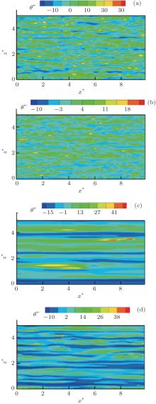
 | Fig. 16. Instantaneous distributions of the near-wall low-temperature streaks for four typical cases in the x– z plane at y+ = 6.9 for (a) BF4-N flow and (b) NF3-N flow, and at y+ = 4.1 for (c) VBF1-N flow and (d) VFBN3-N flow. |
toward the wall as compared with the VBF case. The peak position of the
 | Fig. 17. Profiles of auto-correlation coefficients of temperature difference in the spanwise direction for the four typical fluid cases corresponding to the scenario of Fig. 16. |
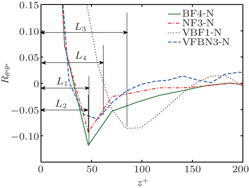
In a turbulent flow with heat transfer, temperature fluctuation and fluctuation of the streamwise velocity component are highly correlated with each other.[28] Related to the near-wall low-speed streaks, the thermal streaky structures can be formed as well near the wall: the high-temperature streak corresponds to the low-speed streak and the low-temperature streak corresponds to the high-speed streak. The instantaneous thermal streaky structures of four typical fluid flows in the x– z plane close to the wall are demonstrated in Fig. 16. It can be seen that the thermal streaky structures for the different cases of BF (Fig. 16(a)), NF (Fig. 16(b)), VBF (Fig. 16(c)), and VFBN (Fig. 16(d)) flows are significantly different: the temperature streaks for the VBF case are the most regular and those for the NF case are the most irregular. More irregular distribution of the thermal streaky structures corresponds to better energy transport performance and larger heat transfer rate. The spanwise spatial intervals of the temperature streaks for the four cases are also estimated through calculating the auto-correlations of temperature difference in the spanwise direction, whose results are plotted in Fig. 17. It can be seen that the spanwise spatial interval of the thermal streaky structures is reduced in the order of VBF, VFBN, BF, and NF flows, corresponding to the fact that the heat transfer ability is enhanced in the order of VBF, VFBN, BF, and NF flows.
From the aforementioned analyses on the characteristics of the mean and fluctuation data of velocity and temperature fields, it is suggested that the VFBN flows have the ability to obtain relative HTE and flow DR. Further, the mechanisms of HTE and flow DR are explored in this section. Quantities contributed to flow resistance and heat transfer, respectively, have been calculated for all the simulated cases in order to reach conclusive understandings of DR and HTE of VFBN flows.
Analysis of the components of flow resistance is started from the momentum equation. The total shear stress can be calculated by Eq. (17) when the flow reaches a statistically steady state[55]

where τ total = (1 − y+ /Reτ ) is the total shear stress. On the right-hand side (RHS) of Eq. (17), the first term is the Reynolds shear stress, the second term is viscous stress, and the third term is elastic stress.
Equation (17) implies that the stress balances of VBF and VFBN flows are changed as compared with the BF case because of the introduction of an extra elastic stress term. Each term on the RHS of Eq. (17) contributes to the total flow resistance. To quantitatively identify the contribution from each of these different terms to the friction factor, the double integration 

In Eq. (18), contribution from the viscous stress does not change at a constant Reynolds number (Rem = Reτ Um/2). The turbulent contribution and elastic contribution are the weighted integrations of the profiles of the Reynolds shear stress and elastic stress with the weight (1 − y* ), respectively.
Utilizing Eq. (18), the ratio of each contribution to the total friction is calculated and shown in Table 2. The friction factor results of the NF flows are not listed in this table because the influences of nanoparticles on flow resistance of BF are not considered in the present simulation for NF flows. The most important finding from Table 2 is that for the viscoelastic fluid flows (VBF and VFBN), the turbulent contribution to the friction factor is greatly reduced as compared with the corresponding Newtonian fluid (BF) flow; although there is an additional elastic contribution, this additional contribution is much smaller in its absolute value than the reduced turbulent contribution, resulting in the occurrence of turbulent DR. Compared with the scenario of the VBF flows, the addition of nanoparticles weakens viscoelasticity of the fluid and so results in an increase in the turbulent contribution to the friction factor and a decreased DR rate.
| Table 2. Contributions to the total friction factor of different simulated cases. |
 | Fig. 18. Contributions to the total friction factor of three typical fluid flows (Reτ = 180). |
To show the DR phenomenon more obviously, the total friction factors and ratios of contributions for the three typical fluids (BF, VBF, and VFBN) are plotted in Fig. 18. At the same Reynolds number, the BF flow has the largest friction factor, of which the turbulent contribution takes a large part; the VBF flow possesses a great reduced total friction factor because of a dramatic decrease in the turbulent contribution; as for the VFBN flow, the turbulent contribution is increased due to the addition of nanoparticles as compared with for the VBF flow, but it is still much lower than that of the BF flow, indicating the flow DR phenomenon.
Taking a similar process to the analysis of flow resistance, the total heat transfer of a turbulent flow is also analyzed based on the energy equation Eq. (7). By decomposing the temperature and velocity in Eq. (7) into average and fluctuation parts and applying assemble average, equation (7) is transformed into the following equation:

Applying the double integration
where

and

Based on the definition of the Nusselt number, equation (20) can be changed into:
where 

is the contribution from the wall-normal turbulent heat flux, and 
Equation (21) is used to calculate each part of different contributions and thus the total heat transfer of a nanofluid turbulent flow is obtained. Unlike the total friction factor balance equation, the total heat transfer is in inverse proportion to the thermal conduction contribution and in proportion to the contributions of the wall-normal turbulent heat flux and thermal dispersion of nanoparticles.
In order to simplify Eq. (21), some definitions are made as follows. R− t = 1/Nu is the total thermal resistance,

is the thermal conduction resistance,

is the turbulent negative thermal resistance (here, the negative thermal resistance, which means a positive effect on heat transfer rate, is introduced because a minus sign exists in front of this term),

is the nanoparticle-effect negative thermal resistance. Then, equation (21) can be simplified into

or

The following definitions are then made for the terms on the RHS of Eq. (23): R% = (R− t/R− cond) × 100% is the ratio of the total thermal resistance to the conductive thermal resistance, R− turb% = (R− turb/R− cond) × 100% is the ratio of turbulent negative thermal resistance to the conductive thermal resistance, R− nano% = (R− nano/R− cond) × 100% is the ratio of nanoparticle-effect negative thermal resistance to the conductive thermal resistance.
The calculated results of these ratios for all the simulated cases are listed in Table 3. The value of R% can represent the heat transfer ability of a tested case: lower value of R% represents an enhancement of heat transfer. For example, the values of R% for the BF flows (BF1-N– BF4-N) are reduced orderly at the increasing Reynolds numbers, representing an HTE at the increasing Reynolds numbers. As seen from the values of R− turb% for BF flows, the increase of R− turb% is the main reason for the enhancement of heat transfer at the increasing Reynolds numbers. For the viscoelastic fluid (VBF1-N– VBF3-N) flows, however, the introduction of viscoelasticity by addition of surfactant or polymer additives into traditional Newtonian-base fluid reduces the value of R− turb/% as compared with the corresponding BF cases, and the value of R− turb/% is reduced with the increase of We (the strengthening of viscoelasticity). Consequently, the total heat transfer is deteriorated for the VBF flows because of the depression of the turbulent contribution. As for water-based nanofluid (NF1-N– NF5-N) flows, and VFBN (VFBN1-N– VFBN5-N) flows, the introduction of nanoparticles induces a nanoparticle-effect negative thermal resistance, and the value of R− nano% is increased with the increase of volume fraction of nanoparticles. Although the value of R− turb% is reduced a little with the increase of volume fraction of nanoparticles, the heat transfer is still enhanced because the increase of R− -nano% is larger than the decrease of R− turb%.
| Table 3. Contributions to heat transfer for different simulated cases. |
According to the analogy theory, if the governing equations of two physical phenomena are similar, the underlying principle of one physical phenomenon can be obtained according to the other corresponding physical phenomenon using a certain similarity criterion. For example, for a turbulent flow with heat transfer, the convective heat transfer correlation can be obtained by the measurement of turbulent flow resistance. The flow friction factor is calculated from the following equation:

and the Chilton– Colburn factor is calculated from the following equation:

For a turbulent flow of the Newtonian fluid with heat transfer, the conventional Colburn-law reads jH/Cf ≈ 0.5, which can be easily found from a heat transfer textbook.
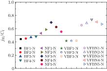
The ratios jH/Cf for the simulated cases are calculated using Eqs. (24) and (25) and shown in Fig. 19. It can be seen that the values of jH/Cf are around 0.5 for the BF flows. But for other cases, values of jH/Cf are significantly deviated from 0.5. jH/Cf is larger than 0.5 for the nanofluid (NF and VFBN) flows, meaning that the overall heat transfer performance is better than the flow characteristic regarding the flow resistance. The value of jH/Cf is lower than 0.5 for the VBF flows, meaning that the flow characteristic is better than the overall heat transfer performance.
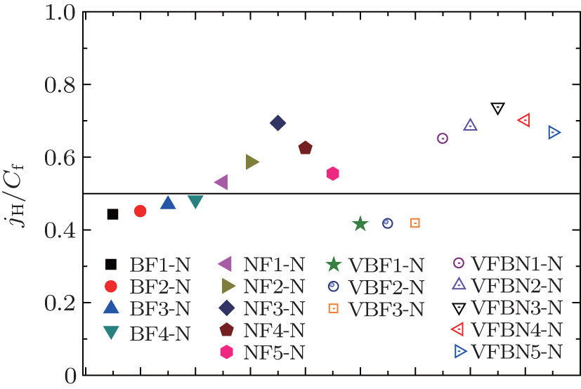 | Fig. 19. Ratios of Chilton– Colburn factor to friction coefficient for different simulated cases. |
The key finding here is that the conventional Colburn-law for the Newtonian-fluid turbulent flows with heat transfer is broken in VFBN turbulent flows toward a desired orientation, i.e., jH/Cf > 0.5. This phenomenon indicates that by utilizing VFBN as a working fluid, it is possible to design a proper energy-conversion system with excellent energy-saving effect, namely, relatively enhanced heat transfer rate and relatively reduced flow drag if the working conditions can be controlled such that jH/Cf > 0.5.
In this work, we perform the DNSs for turbulent channel flows of VFBN based on our previously proposed thermal dispersion model for a nanofluid turbulent flow. Using the DNS database, the mean and fluctuation features of the velocity and temperature fields in the simulated flows, heat transfer contributions, flow resistance contributions, and analogy between flow resistance and heat transfer characteristics are analyzed. Some conclusions can be drawn from the present study as follows.
(i) Results for the mean features of flow and heat transfer properties for the simulated cases show that the present DNSs can capture the main characteristics of the NF, VBF, and VFBN turbulent flows which appear in experiment. This indicates that the present DNS procedure is reliable.
(ii) By analyzing the characteristics of the near-wall low-speed streaks and near-wall thermal streaks in BF, NF, VBF, VFBN flows, it can be concluded that VFBN flows take on more regular low-speed streaks than the BF flows, reflecting a turbulent DR effect, while present more irregular thermal streaks than the VBF flows, reflecting an HTE effect.
(iii) Analyses of the values of jH/Cf for the simulated BF, NF, VBF, and VFBN flows show that the nanofluid flows possess better overall heat transfer performances than flow characteristics regarding the flow resistance.
(iv) The mechanism of turbulent DR of VFBN flows can be summarized as follows. Although the viscoelasticity in the VFBN flow makes an additional elastic contribution to the total friction factor, it can also dramatically depress the turbulent contribution to the total friction factor; the decrease of the turbulent contribution is much larger than the elastic contribution, which eventually results in flow DR.
(v) The mechanism of HTE of NF or VFBN flows can be summarized as follows. Considering the thermal dispersion of nanoparticles, an extra nanoparticle-effect negative thermal resistance is introduced into the NF and VFBN flows, which enhances convective heat transfer; meanwhile, the thermal dispersion effect also slightly reduces the turbulent negative thermal resistance, but this reduction is smaller than the extra nanoparticle-effect negative thermal resistance.
| 1 |
|
| 2 |
|
| 3 |
|
| 4 |
|
| 5 |
|
| 6 |
|
| 7 |
|
| 8 |
|
| 9 |
|
| 10 |
|
| 11 |
|
| 12 |
|
| 13 |
|
| 14 |
|
| 15 |
|
| 16 |
|
| 17 |
|
| 18 |
|
| 19 |
|
| 20 |
|
| 21 |
|
| 22 |
|
| 23 |
|
| 24 |
|
| 25 |
|
| 26 |
|
| 27 |
|
| 28 |
|
| 29 |
|
| 30 |
|
| 31 |
|
| 32 |
|
| 33 |
|
| 34 |
|
| 35 |
|
| 36 |
|
| 37 |
|
| 38 |
|
| 39 |
|
| 40 |
|
| 41 |
|
| 42 |
|
| 43 |
|
| 44 |
|
| 45 |
|
| 46 |
|
| 47 |
|
| 48 |
|
| 49 |
|
| 50 |
|
| 51 |
|
| 52 |
|
| 53 |
|
| 54 |
|
| 55 |
|