Cheng Sheng-Yi, Liu Wen-Jin, Chen Shan-Qiu, Dong Li-Zhi, Yang Ping, Xu Bing†. Comparison between iterative wavefront control algorithm and direct gradient wavefront control algorithm for adaptive optics system. Chinese Physics B, 24(8): 084214
Permissions
Comparison between iterative wavefront control algorithm and direct gradient wavefront control algorithm for adaptive optics system
Cheng Sheng-Yia),b),c), Liu Wen-Jina),c), Chen Shan-Qiua),c), Dong Li-Zhia),c), Yang Pinga),c), Xu Bing†a)
Laboratory on Adaptive Optics, Institute of Optics and Electronics, Chinese Academy of Sciences, Chengdu 610209, China
Key Laboratory on Adaptive Optics, Chinese Academy of Sciences, Chengdu 610209, China
University of the Chinese Academy of Sciences, Beijing 100049, China
*Project supported by the National Key Scientific and Research Equipment Development Project of China (Grant No. ZDYZ2013-2), the National Natural Science Foundation of China (Grant No. 11173008), and the Sichuan Provincial Outstanding Youth Academic Technology Leaders Program, China (Grant No. 2012JQ0012).
Abstract
Among all kinds of wavefront control algorithms in adaptive optics systems, the direct gradient wavefront control algorithm is the most widespread and common method. This control algorithm obtains the actuator voltages directly from wavefront slopes through pre-measuring the relational matrix between deformable mirror actuators and Hartmann wavefront sensor with perfect real-time characteristic and stability. However, with increasing the number of sub-apertures in wavefront sensor and deformable mirror actuators of adaptive optics systems, the matrix operation in direct gradient algorithm takes too much time, which becomes a major factor influencing control effect of adaptive optics systems. In this paper we apply an iterative wavefront control algorithm to high-resolution adaptive optics systems, in which the voltages of each actuator are obtained through iteration arithmetic, which gains great advantage in calculation and storage. For AO system with thousands of actuators, the computational complexity estimate is about O( n2) ∼ O( n3) in direct gradient wavefront control algorithm, while the computational complexity estimate in iterative wavefront control algorithm is about O( n) ∼ ( O( n)3/2), in which n is the number of actuators of AO system. And the more the numbers of sub-apertures and deformable mirror actuators, the more significant advantage the iterative wavefront control algorithm exhibits.
PACS:
42.68.Wt; 95.75.Qr; 07.05.Tp
Keyword:
adaptive optics; iterative wavefront control algorithm; direct gradient wavefront control algorithm
Adaptive optics (AO) is a technique that was conceived to compensate in real time for the phase perturbations introduced by atmospheric turbulence.[1, 2] At present, AO systems have been used in many fields, such as improving laser beam quality, [3– 8] correcting the errors in astro-observation brought by atmospheric disturbances, [9– 12] researching on ocular aberration, etc. The standard and most used wavefront control algorithm for AO system is a direct gradient wavefront control algorithm, which is based on a matrix-vector multiplication of the relational matrix from deformable mirror (DM) to Hartmann wavefront sensor (WFS) and the slope vector measured by WFS. But as the number of actuators of AO system increases, the computational complexity of direct gradient wavefront control algorithm becomes much greater. This algorithm cannot be achieved by present data processing system because of the large amount of calculation. In order to solve the problem, Luc et al.[13, 14] and Eric and Michel[15] proposed preconditioned conjugate gradient algorithm and minimum variance algorithm respectively. But in both of the methods, Zernike mode coefficients of reconstructed wavefront are obtained through iteration arithmetic by using the wavefront slope data of sub-apertures in WFS first, and then the control voltages of DM actuators are calculated according to the relational matrix from Zernike mode coefficients to DM actuators. In this paper, we provide an iterative wavefront control algorithm for AO system, and the control voltages of the DM actuators are directly calculated by using the iteration arithmetic based on the slope data detected by the WFS, so it leaves out the calculating of Zernike mode coefficients and improves the efficiency of wavefront control process. When calculating voltages by using the iteration arithmetic, the iterative matrix is a sparse matrix. Iterative matrix with high sparseness can not only lower the computational complexity of the control algorithm, but also reduce the storage space occupied.[14– 18]
The rest of this paper is arranged as follows. In Section 2, we introduce the direct gradient wavefront control algorithm. In Section 3, we introduce the iterative wavefront control algorithm. In Section 4, the principle of solution to iterative wavefront control algorithm is deduced and then the equation of computational complexity is given. In Section 5, the sparsity of iterative matrix in iterative wavefront control algorithm is analyzed. Afterwards, the computational complexity comparison between the direct gradient wavefront control algorithm and the iterative wavefront control algorithm is presented in Section 6. And finally some conclusions are drawn from the present study in Section 7.
2. Direct gradient wavefront control algorithm
Direct gradient wavefront control algorithm uses the control voltage of each DM actuator as the calculation target of the wavefront control. According to the influence on slope data of sub-apertures when each actuator is applied to by unit voltage, the relational matrix from DM actuators to sub-apertures in WFS is established.[19]
Suppose input voltage signal Vj is the control voltage applied to the actuator No. j, the average wavefront slope of the sub-apertures in WFS is produced as follows:[19]
where Rj(x, y) is the influence function of the actuator No. j of DM, t is the number of the actuator, m is the number of sub-aperture, and Si is the normalized area of sub-aperture i. When the control voltage functions in a right range, sub-aperture gradient and the drive voltage form a linear relation. Equation (1) can be presented as follows:
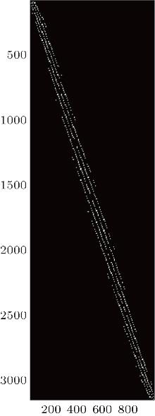
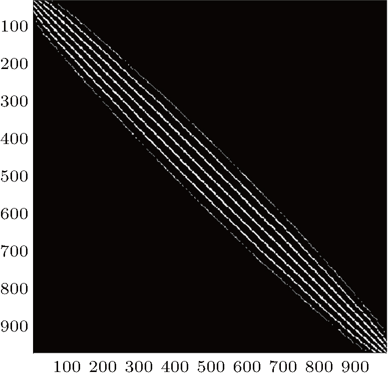
where Rxy is the slope response matrix from DM to WFS. In a general case, the matrix is obtained in experiment. Taking 991-actuator AO system for example. Figure 1 shows the slope response matrix of the 991-actuator AO system. The positions marked by white lines indicate the non-zero elements of the matrix, while the black area indicates the zero elements. When the elements in slope response matrix are less than one percent of the maximum one, the influence of these elements on wavefront control can be omitted. So these elements are treated as being zero elements.
Fig. 1. Slope response matrix of 991-actuator AO system.
In the wavefront control process with using direct gradient wavefront control algorithm, the inverse matrix of Rxy is used as control matrix. The control relation is expressed as follows:
where is the control matrix of direct gradient wavefront control algorithm in wavefront control process, g is the sub-aperture slope information detected by WFS, v is the voltage applied to the actuator of DM, which is calculated by control system. Figure 2 provides the of the 991-actuator AO system. The white area indicates the non-zero elements of the control matrix, while the black area represents the zero elements. It is obvious that the control matrix is almost occupied by non-zero elements.
Comparison between Fig. 1 and Fig. 2 shows that slope response matrix is a sparse matrix, while control matrix is a non-sparse matrix. As is the generalized inverse matrix of Rxy, then an analysis about is conducted. The general principle is used to obtain the inverse matrix as
According to Eq. (3), the equation of direct gradient wavefront control algorithm can be expressed as
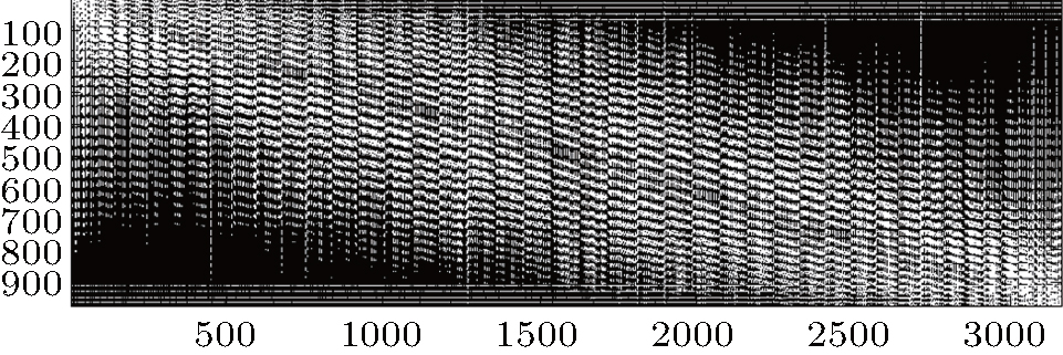
Figure 3 provides the of 991-actuator AO system. In Fig. 3, the white lines indicate the non-zero elements of , the black area represents the zero elements of . is the iterative matrix in iterative wavefront control algorithm. It can be seen that is also a sparse matrix.
Fig. 3. Iterative matrix of 991-actuator AO system.
Because is the transposed matrix of Rxy, is also a sparse matrix. In Eq. (6), both and are sparse matrixes, therefore both sides of Eq. (6) are sparse matrix vector multiplication. Iterative wavefront control algorithm solves the voltages applied to DM actuators in the way of iteration based on Eq. (6). The computational complexity of sparse matrix vector multiplication is far smaller than that of general matrix vector multiplication, [16– 18] thus, using the iterative wavefront control algorithm to obtain the voltages applied to the DM actuators can greatly reduce the storage space of wavefront control algorithm.
4. Computational complexity of iterative wavefront control algorithm
Equation (6) can be regarded as the form of Ax = b: where is A, is b, the voltage signal v is x (A ∈ Rn × n, b ∈ Rn). Using conjugate gradient method, [20] for any initial vector x0, the first search direction p0 is chosen as
The system of conjugate vectors {pk} with pk ≠ 0 (k = 0, 1, 2, … ) possesses the following property:
For the given initial approximate vector x0, suppose p0 = − r0 = − (Ax0 − b), when k = 0, 1, 2, … , then the iterative wavefront control algorithm will be
In the calculation process, if rk+ 1 = 0, then xk+ 1 is the solution of Ax = b.
For a real-time AO system, the residual wavefront is detected by WFS, so the slope information we obtained is only relevant to the residual wavefront. The voltages calculated by iterative wavefront control algorithm are only the variation of voltages which are applied to DM actuators in two successive wavefront control processes. In a real-time system, the DM shape is in continuous change, the voltages applied to DM actuators between two successive wavefront control processes change very little. Therefore, in the wavefront control process by using iterative wavefront control algorithm, the initial variation of voltages can be assigned to zero vector. In this way, iterative wavefront control algorithm can converge quickly, so the iterative times of iterative wavefront control algorithm will decrease and the computational complexity will be reduced.
Let n be the number of DM actuators, m the number of sub-apertures in WFS of AO system, c the number of non-zero elements of iterative matrix, and k the iteration times of iterative wavefront control algorithm, according to operation process in real system, then the multiplication computational complexity of the iterative wavefront control algorithm will be calculated as
Addition computational complexity is
The multiplication computational complexity and addition computational complexity of direct gradient wavefront control algorithm are both
To make a computational complexity comparison between direct gradient wavefront control algorithm and iterative wavefront control algorithm, the number of the non-zero elements c in iterative matrix and the iterative times k of iterative wavefront control algorithm must be analyzed first.
5. Analysis of the iterative matrix sparsity
In the wavefront control process with using the iterative wavefront control algorithm, if the iterative matrix is a non-sparse matrix or a matrix in low sparsity, the advantage of iterative wavefront control algorithm disappears. Therefore, when making the complexity comparison between direct gradient wavefront control algorithm and iterative wavefront control algorithm, the sparsity of iterative matrix must be first analyzed. We choose 8 different groups of AO systems which are listed in Table 1.
Table 1.
Table 1.
Table 1. Selected 8 different groups of AO systems.
The number of DM actuators (n)
The number of sub-aperture in WFS (m)
The number of non-zero element of iterative matrix (c)
The amount of element of iterative matrix
61
14× 14
1399
3721
91
17× 17
2245
8281
169
23× 23
4115
28561
265
24× 24
6827
70225
379
32× 32
9801
143641
529
34× 34
14615
279841
685
37× 37
18043
469225
979
45× 45
27241
958441
Table 1. Selected 8 different groups of AO systems.
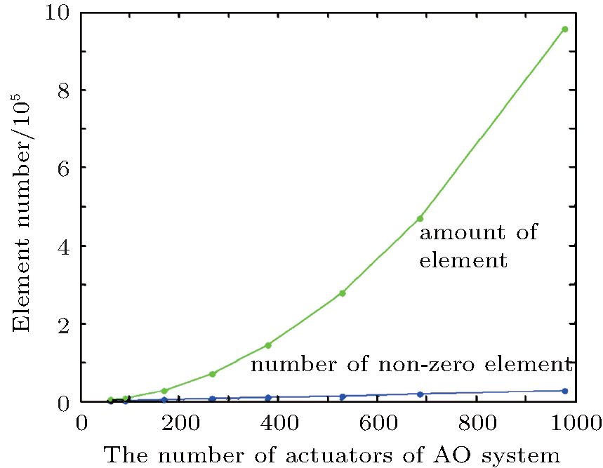
In order to visually display the sparsity of iterative matrix, a comparison can be made among the 8 groups of AO system. As the number of actuators of AO system increases, the change trends of total element number and non-zero element number of iterative matrix are shown in Fig. 4.
Fig. 4. Change trends of total element number and non-zero element number of iterative matrix.
As the number of actuators of AO system increases, the total elements of iterative matrix increases quickly, while the non-zero elements increase extremely slowly.
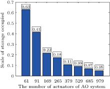
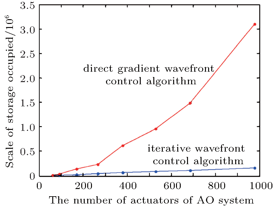
Based on the eight groups of AO systems, a comparison is made between the storage space occupied by direct gradient wavefront control algorithm and that by iterative wavefront control algorithm. Figure 5 shows the change trends of the storage space occupied by direct gradient wavefront control algorithm and that by iterative wavefront control algorithm with the increase of AO system actuators. Figure 6 shows the ratios of the space occupied by iterative wavefront control algorithm to the space occupied by direct gradient wavefront control algorithm.
Fig. 6. Rations of the storage space occupied by iterative wavefront control algorithm to the storage space occupied by direct gradient wavefront control algorithm.
From Fig. 5, it can be seen that the storage space occupied by direct gradient wavefront control algorithm apparently grows while the storage space occupied by iterative wavefront control algorithm grows slowly with the increase of the number of AO system actuators. From Fig. 6, the ratio of the storage space occupied by iterative wavefront control algorithm to the storage space occupied by direct gradient wavefront control algorithm becomes smaller and smaller with the increase of the number of AO system actuators. Compared with the direct gradient wavefront control algorithm, the iterative wavefront control algorithm is apparently advantageous in storage space. When the number of AO system actuators approaches to 1000, the storage space occupied by direct gradient wavefront control algorithm is 20 times as large as that occupied by iterative wavefront control algorithm. Therefore, it can be deduced that when the number of AO system actuators approaches to 104, the storage space occupied by direct gradient wavefront control algorithm will be hundreds, even thousands of times as large as that occupied by iterative wavefront control algorithm. It means that for the AO system with a large number of actuators, the communication bandwidth required by direct gradient wavefront control algorithm is hundreds, even thousands of times compared with that required by iterative wavefront control algorithm.
6. Computational complexity comparison between iterative wavefront control algorithm and direct gradient wavefront control algorithm
The occupied storage space is a significant factor to weight a wavefront control algorithm. Another more significant factor is the computational complexity of wavefront control algorithm. This section chiefly compares iterative wavefront control algorithm with direct gradient wavefront control algorithm in the sense of computational complexity.
In experiment, the input wavefront is the dynamic wavefront with aberration of defocus. For the 8 groups of AO systems in Table 1, equations (10) and (11) can be used to calculate the multiplication computational complexity and addition computational complexity of iterative wavefront control algorithm. Equation (12) can be used to calculate the multiplication computational complexity and addition computational complexity of direct gradient wavefront control algorithm. The multiplication computational complexity and addition computational complexity are approximate in iterative wavefront control algorithm, while they are equal in direct gradient wavefront control algorithm. Therefore, it is enough to make a comparison of multiplication computational complexity between the two algorithms. The comparison is shown in Table 2.
Table 2.
Table 2.
Table 2. Computational complexity comparison between iterative wavefront control algorithm and direct gradient wavefront control algorithm.
Relational matrix of different adaptive optics systems
Maximum iteration times of iterative algorithm
Multiplication computational complexity of iterative algorithm
Multiplication computational complexity of direct control algorithm
296× 61
15
29765
18056
442× 91
18
55850
40222
842× 169
20
113624
142298
896× 265
22
203926
237440
1624× 379
25
331005
615496
1808× 529
30
580554
956432
2170× 685
32
771464
1486450
3162× 979
48
1711724
3095598
Table 2. Computational complexity comparison between iterative wavefront control algorithm and direct gradient wavefront control algorithm.
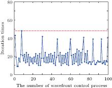
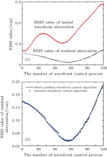
Taking the AO system in the eighth row of Table 2 for example, the wavefront control effects of the direct gradient wavefront control algorithm and the iterative wavefront control algorithm are firstly analyzed. Figure 7 shows the distribution of iteration times of the iterative wavefront control algorithm in 100 dynamic wavefront control processes. Figure 8 shows the comparison between the RMS values of the residual wavefront aberration in 100 dynamic wavefront control processes, obtained respectively by using iterative wavefront control algorithm and direct gradient wavefront control algorithm.
Fig. 8. Comparison of RMS value of the residual wavefront aberration between the iterative wavefront control algorithm and the direct gradient wavefront control algorithm.
In Fig. 7, it can be seen that the iteration times of the iterative wavefront control algorithm are usually below 48 in the 979-actuator AO system. Therefore, the maximum of iteration times of the 979-actuator AO system in the eighth row of Table 2 is 48.
In Fig. 8(a), the upper curve represents the RMS value of the initial wavefront aberration, and the two lower curves refer to the RMS values of the residual wavefront aberration in dynamic wavefront control process, obtained respectively by using iterative wavefront control algorithm and direct gradient wavefront control algorithm. The two lower curves are nearly identical. In Fig. 8(a), it is evident that both the wavefront control algorithms can reduce the wavefront aberration to a certain extent. In order to clearly display the difference in wavefront control effect between the two algorithms, the two lower curves in Fig. 8(a) are shown in Fig. 8(b). In Fig. 8(b), it is obvious that the control effects of the iterative wavefront control algorithm and the direct gradient wavefront control algorithm are nearly the same.
In order to visually express the comparison between iterative wavefront control algorithm and direct gradient wavefront control algorithm, the figure about the complexity comparison is drawn as follows.
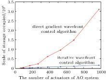
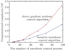
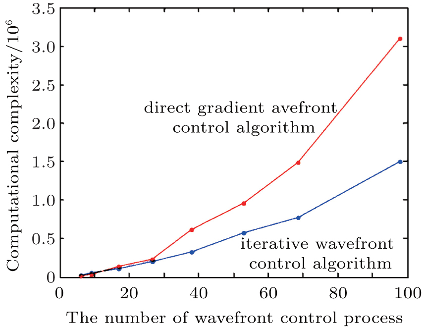
In Fig. 9, the computational complexity of direct gradient wavefront control algorithm is lower than that of iterative wavefront control algorithm when the number of actuators of AO system is small. But with the increase of the number of actuators of AO system, the computational complexity of direct gradient wavefront control algorithm increases more obviously than that of iterative wavefront control algorithm. In order to assess the two algorithms in AO system with more actuators, the variations of the two computational complexity estimate curves with the number of AO system actuators are shown in Fig. 10.
Fig. 9. Computational complexity comparison between iterative wavefront control algorithm and direct gradient wavefront control algorithm.
In Fig. 10, n is the number of actuators of AO system. We can obtain the computational complexity estimate is about O(n2.043) in the direct gradient wavefront control algorithm, while the computational complexity estimate in the iterative wavefront control algorithm is about O(n1.588). And when the number of actuators of AO system grows to about 1000, the computational complexity of direct gradient wavefront control algorithm is one time more than that of iterative wavefront control algorithm. With this trend, when the number of actuators of AO system becomes greater, the multiple will be tens, even hundreds of times.
Fig. 10. Computational complexity estimates of iterative wavefront control algorithm and direct gradient wavefront control algorithm.
7. Conclusions
We introduce the iterative wavefront control algorithm, a wavefront control algorithm chiefly used in the AO system with a large number of actuators. And the more the actuators, the more obvious its advantage is. This paper illustrates the advantage of iterative wavefront control algorithm from two aspects.
The obvious advantage of iterative wavefront control algorithm is that it reduces the occupied storage of AO system. Compared with direct gradient wavefront control algorithm, when the number of actuators grows to 1000, iterative wavefront control algorithm only takes 5 percent of its storage. For a larger number of actuators of AO system, the advantage of iterative wavefront control algorithm in saving storage space will be more obvious.
Another significant advantage is that for an AO system with a large number of actuators, the computational complexity of iterative wavefront control algorithm is far smaller than that of direct gradient wavefront control algorithm. With the increase of the actuator number in the AO system, the computational complexity of the direct gradient wavefront control algorithm grows rapidly, while the computational complexity of the iterative wavefront control algorithm grows slowly. Finally we show that the computational complexity estimate of iterative wavefront control algorithm approaches to O(n1.5), while the computational complexity estimate of direct gradient wavefront control algorithm exceeds O(n2). Although this paper has only done the research about AO system within 1000 actuators, it is still meaningful for the AO system with thousands of actuators.
JiangW and LiH1990Adaptive Optics and Optical Structures, Proc. SPIEMarch 1, 1990The Hague, Netherland s82[Cited within:2]
20
ZhuY, RaoL, YanT, ZhangJ and LiB2010Matrix Analysis and Calculation(Vol. 9)BeijingNational Defense Industry Press160(in Chinese)[Cited within:1]
1
1991
0.0
0.0
... [1,2] At present, AO systems have been used in many fields, such as improving laser beam quality,[3#cod#x2013 ...
1
2006
0.0
0.0
... [1,2] At present, AO systems have been used in many fields, such as improving laser beam quality,[3#cod#x2013 ...
1
2012
0.0
0.0
... [1,2] At present, AO systems have been used in many fields, such as improving laser beam quality,[3#cod#x2013 ...
1
2008
0.0
0.0
1
2013
0.0
0.0
1
2012
0.0
0.0
1
2014
0.0
0.0
1
2010
0.0
0.0
... 8] correcting the errors in astro-observation brought by atmospheric disturbances,[9#cod#x2013 ...
1
2009
0.0
0.0
... 8] correcting the errors in astro-observation brought by atmospheric disturbances,[9#cod#x2013 ...
1
2009
0.0
0.0
1
2003
0.0
0.0
1
2002
0.0
0.0
... 12] researching on ocular aberration, etc ...
1
2002
0.0
0.0
... [13,14] and Eric and Michel[15] proposed preconditioned conjugate gradient algorithm and minimum variance algorithm respectively ...
2
2003
0.0
0.0
... [13,14] and Eric and Michel[15] proposed preconditioned conjugate gradient algorithm and minimum variance algorithm respectively ...
... [14#cod#x2013 ...
1
2010
0.0
0.0
... [13,14] and Eric and Michel[15] proposed preconditioned conjugate gradient algorithm and minimum variance algorithm respectively ...
1
2004
0.0
0.0
... The computational complexity of sparse matrix vector multiplication is far smaller than that of general matrix vector multiplication,[16#cod#x2013 ...
1
2011
0.0
0.0
2
2004
0.0
0.0
... 18] ...
... 18] thus, using the iterative wavefront control algorithm to obtain the voltages applied to the DM actuators can greatly reduce the storage space of wavefront control algorithm ...
2
1990
0.0
0.0
... [19] ...
... j, the average wavefront slope of the sub-apertures in WFS is produced as follows:[19] ...
1
2010
0.0
0.0
... Using conjugate gradient method,[20] for any initial vector x0, the first search direction p0 is chosen as ...
Comparison between iterative wavefront control algorithm and direct gradient wavefront control algorithm for adaptive optics system
[Cheng Sheng-Yia),b),c), Liu Wen-Jina),c), Chen Shan-Qiua),c), Dong Li-Zhia),c), Yang Pinga),c), Xu Bing†a)]


 ]
]