


Fractional-order systems without equilibria: The first example of hyperchaos and its application to synchronization
[Cafagna Donato† , Grassi Giuseppe
‡ ]
, Grassi Giuseppe|
|


†Corresponding author. E-mail: donato.cafagna@unisalento.it
‡Corresponding author. E-mail: giuseppe.grassi@unisalento.it
A challenging topic in nonlinear dynamics concerns the study of fractional-order systems without equilibrium points. In particular, no paper has been published to date regarding the presence of hyperchaos in these systems. This paper aims to bridge the gap by introducing a new example of fractional-order hyperchaotic system without equilibrium points. The conducted analysis shows that hyperchaos exists in the proposed system when its order is as low as 3.84. Moreover, an interesting application of hyperchaotic synchronization to the considered fractional-order system is provided.
The concept of fractional calculus was proposed by Leibniz in the early 17th century. For a long time, fractional calculus has been unexplored due to its intrinsic complexity and the lack of an intuitive geometrical and physical interpretation.[1– 3] It has only been during the last few decades that physicists and engineers have understood that problems encountered in viscoelasticity, dielectric polarization, electromagnetic waves, quantitative finance, electrical circuit theory, and control systems can be more accurately described using fractional calculus.[4, 5]
More recently, many researchers have shown growing interest in the study of chaos in fractional-order dynamical systems.[6, 7] Specifically, great attention has been focused on chaotic (only one positive Lyapunov exponent) and hyperchaotic (two or more positive Lyapunov exponents) behaviors of nonlinear fractional systems.[8– 15] Some examples include the fractional chaotic Chua’ s circuit, [8, 9] the fractional chaotic Lorenz system, [10] the fractional chaotic Chen system, [11, 12] the fractional hyperchaotic Rö ssler system, [13] and the fractional systems generating multi-scroll and multi-wing attractors.[14, 15]
It is worth noting that all the above mentioned fractional systems are characterized by one or more equilibrium points. However, a very challenging topic is about the study of fractional-order systems without equilibrium points. Note that the presence of chaos in nonlinear systems without equilibria is very surprising since they can have neither homoclinic nor heteroclinic orbits, [16] and thus the Shilnikov theorem cannot be applied.[17] In this regard, referring to the presence of chaos in fractional-order systems with no equilibria, only very few papers have been published.[18– 20] On the other hand, referring to the presence of hyperchaos in fractional-order systems without equilibria, to the best of our knowledge, no paper has been published in the literature so far.
Based on these considerations, this paper aims to bridge the gap by introducing a new example of a fractional-order hyperchaotic system without equilibrium points. The conducted analysis shows that the proposed system exhibits hyperchaotic attractors when the system order is as low as 3.84. Moreover, an application of hyperchaotic synchronization to the considered fractional-order system is provided.
The rest of this paper is organized as follows. In Section 2 the fundamentals of fractional calculus and the predictor-corrector method of solving fractional differential equations are briefly reported. In Section 3 the considered fractional-order system with no equilibria is introduced. The proposed system, which represents the fractional-order counterpart of the integer-order system without equilibria reported in Ref. [21], is studied by using the predictor– corrector algorithm. An attractor is found when the order of the derivative is q = 0.96 and its hyperchaotic nature is confirmed by the application of a recent numerical method.[22] In Section 4 a deep analysis of the considered fractional system is conducted, in order to better understand its novel and yet unexplored dynamical properties. Finally, in Section 5 an example of observer-based synchronization involving the considered hyperchaotic fractional-order system is described in detail.
The Riemann– Liouville fractional integral operator 

where Γ (q) is the Gamma function, with 
For γ > − 1 and a real constant C, two fundamental properties of the integral operator 

Different definitions of fractional differential operators have been proposed in Ref. [23]. In this manuscript the Caputo differential operator 
where m – 1 < q ≤ m and m ∈ N (i.e., m = ceil(q)).[24] Two fundamental properties of the differential operator 


Based on Caputo’ s definition (4), the following general form of fractional-order differential equation is considered:

It has been demonstrated that the initial value problem (7) is equivalent to a Volterra integral equation, [25]
in the sense that a continuous function solves Eq. (8) if and only if it solves Eq. (7).
Now, the Volterra integral equation (8) is solved by applying the predictor-corrector iterative algorithm, which belongs to the Adams– Bashforth– Moulton (ABM) scheme. In particular, the product trapezoidal quadrature formula is used to replace the integral in Eq. (8). By taking 0 ≤ t ≤ T and by setting h = T/N (N ∈ Z+ ), tn = nh, n = 0, 1, … , N, equation (8) can be discretized as[25]
where

Equation (9) can be rewritten as[25]
The solution via the ABM method is carried out by first predicting (x(p)(tn+ 1)) using the explicit Adams– Bashforth formula and then correcting (x(tn+ 1)). Thus, equation (11) is solved as[25]

where

The error of the algorithm is

with (j = 0, 1, … , N), where ρ = Min(2, 1 + q).[26]
Referring to hyperchaos in integer-order dynamical systems, [27– 29] very recently the first example of a four-dimensional (4D) hyperchaotic system with no equilibrium has been given in Ref. [21]. The integer-order differential equations of the system in Ref. [21] are
where a, b, and c are constant parameters of the system (15). As shown in Ref. [21], system (15) has no equilibrium and it has no dynamical behaviors such as pitchfork bifurcation, Hopf bifurcation, etc. When a = 8, b = − 2.5, and c = − 30, the system has the hyperchaotic attractor plotted in Ref. [21], with the Lyapunov exponents given by λ 1 = 0.87, λ 2 = 0.03, λ 3 = 0.00, and λ 4 = − 1.01, which show that the system is hyperchaotic. Note that the presence of hyperchaos in such a system is very surprising since it can have neither homoclinic nor heteroclinic orbits, [16] and thus the Shilnikov theorem[17] cannot be used to verify the chaos.
Referring to fractional-order hyperchaotic systems without equilibria, to the best of our knowledge, no paper has been published in the literature so far. Based on this consideration, this study bridges the gap by introducing the first example of fractional hyperchaos. Specifically, the equations of the proposed system, which represents the fractional-order counterpart of system (12), are

where * Dq denotes the Caputo fractional operator defined in Eq. (4) with initial time t0 = 0, order q ∈ (0, 1) and a ≠ 0.[24] Like the integer order system (15) and as discussed in Section 4, the proposed system (16) has no equilibrium points for any value of the parameters a, b, and c. By applying the predictor-corrector algorithm described in Section 2, the solution of the fractional system (16) can be written as
in which the predicted variables are
where α j, n+ 1 and β j, n+ 1 are given by Eqs. (10) and (14), respectively.
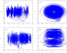
By considering the parameter values a = 8, b = − 2.5, and c = − 30, the discretized equations (17) and (18) are calculated for several values of order 0 < q < 1. A remarkable finding of this paper is that hyperchaos exists in the proposed fractional-order system without equilibrium points when the value of q is as low as 0.96. The phase portraits of the hyperchaotic attractor are shown in Figs. 1 and 2 for the sets of initial conditions given by (0.1, 0.1, 0.1, 0.1) and (0.12, 0.12, 0.12, 0.12), respectively.
 | Fig. 1. Hyperchaotic attractors of the fractional-order system without equilibrium points (16) with q = 0.96 and initial conditions (0.1, 0.1, 0.1, 0.1): (a) attractor in the (x, w)-plane, (b) attractor in the (y, w)-plane, (c) attractor in the (z, w)-plane, (d) attractor in the (y, z)-plane. |
The hyperchaotic natures of the attractors reported in Figs. 1 and 2 are confirmed by computing the Lyapunov exponents through using the technique based on the recent paper.[22] Note that, while other numerical methods (like the Wolf algorithm) only give an estimation of the largest Lyapunov exponent, the algorithm proposed in Ref. [22] is the only one (to the best of our knowledge) that is able to provide the entire spectrum of Lyapunov exponents in fractional-order systems. Specifically, in Ref. [22] an application of a transformation technique (i.e., the Differential Transform Method) to fractional differential equations is exploited for calculating the Lyapunov exponents. In particular, for q = 0.96 and for the previous sets of initial conditions, i.e., (0.1, 0.1, 0.1, 0.1) and (0.12, 0.12, 0.12, 0.12), the obtained spectra are (λ 1 = 0.91, λ 2 = 0.19, λ 3 = 0, λ 4 = − 1.37) and (λ 1 = 0.89, λ 2 = 0.21, λ 3 = 0, λ 4 = – 1.54), respectively. These spectra include two positive values, confirming the hyperchaotic natures of the attractors reported in Figs. 1 and 2 when q is as low as 0.96.
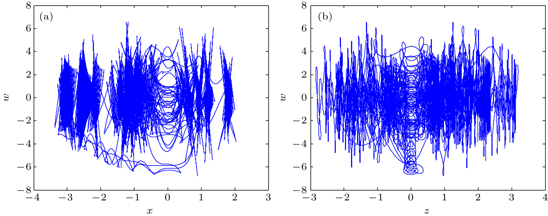 | Fig. 2. Hyperchaotic attractors of the fractional-order system without equilibrium points (16) with q = 0.96 and initial conditions (0.12, 0.12, 0.12, 0.12): (a) attractor in the (x, w)-plane, (b) attractor in the (z, w)-plane. |
In order to further investigate the dynamic behaviour of the system (16) for other values of the order q, the spectrum of the Lyapunov exponents is computed as a function of parameter q. The spectrum (see Fig. 3) shows that the two largest Lyapunov exponents remain positive when q varies in the interval [0.96, 1]. The plot in Fig. 3 indicates that the proposed fractional-order system (16) is hyperchaotic for different values of parameter q. Note that when q = 1, the plot is in agreement with the results given in Ref. [21] for the integer-order counterpart of the proposed system (16).
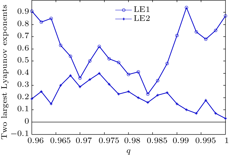 | Fig. 3. Plots of the two largest Lyapunov exponents of system (16) versus fractional-order q. |
An analysis of the considered fractional-order system (16) is conducted in order to better understand its dynamical properties as well as its hyperchaotic behavior. For this purpose, it is worth recalling that given a dynamical systems, a bifurcation occurs when a small smooth change made to be a parameter value (the bifurcation parameter) causes a sudden qualitative or topological change in its behavior. In particular, a local bifurcation occurs when a parameter change causes the stability of an equilibrium to change. On the other hand, a global bifurcation occurs when an invariant set, such as a periodic orbit, collides with an equilibrium.[30]
Since the presence of equilibrium plays a key role in the occurring of bifurcations, it is important to check whether there exists a parameter value that makes an equilibrium point to appear in the considered system (16). This check is carried out by taking * Dq (· ) = 0 in system (16), i.e.,


From Eqs. (19a) and (19c), it can be readily deduced that constraint y = 0 is inconsistent with y = ± 1, indicating that system (16) has no equilibrium for any value of parameters a, b, and c. In other words, it is impossible for an equilibrium point to appear in system (16), for any choice of parameters a, b, and c. As a consequence, any change in parameters a, b, and c can generate neither local nor global bifurcations in system (16), indicating that a or b or c cannot be considered as a bifurcation parameter. Such a result is in perfect accordance with the results found in Ref. [21] for the corresponding integer-order hyperchaotic system.
Recall that very recently, chaotic systems without equilibrium points have been categorized as chaotic systems with hidden attractors[31– 33] since their basins of attraction do not intersect with small neighborhoods of any equilibrium points and, consequently, there is no regular way to predict the existence nor coexistence of hidden attractors. The proposed system (16) belongs to the class of chaotic systems with hidden attractors. However, the considered system (16) has a different behavior from other chaotic systems with hidden attractors found in the literature, since these systems are constructed by adding a tiny perturbation to a simple chaotic flow having a single equilibrium or a line equilibrium.[34] For example, the authors of Ref. [35] applied a tiny perturbation to the Sprott E system to change the stability of its single equilibrium to a stable one. In the same way, a tiny perturbation makes the Sprott D system with a degenerate equilibrium have no equilibrium.[36] In addition, the authors of Ref. [37] have implemented a systematic search algorithm to find a catalog of chaotic flows with no equilibria, whereas the authors of Ref. [38] have carried out a series of simple chaotic flows with a line of equilibria. In conclusion, the dynamic behavior of the proposed fractional-order system (16) represents a novelty in the literature, since the absence of equilibria is a structural property of the system which is not affected by any tiny perturbation of a single or line equilibrium.
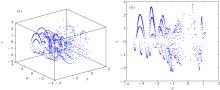
In order to further investigate the dynamic properties of the proposed 4D fractional-order system (16), the Poincare map and the power spectrum are constructed. In particular, the Poincare map is useful for understanding the system dynamics, since it preserves many properties of the original system but has a lower-dimensional state space. By taking w = 0 as the crossing plane, figure 4(a) shows the Poincaré map in the three-dimensional (3D) (x, y, z)-space, whereas figure 4(b) shows the Poincaré map in the two-dimensional (2D) (x, z)-plane. Note the presence of several distinct sets of points in the Poincare map, clearly indicating the presence of rich chaotic dynamics in the proposed fractional-order system.
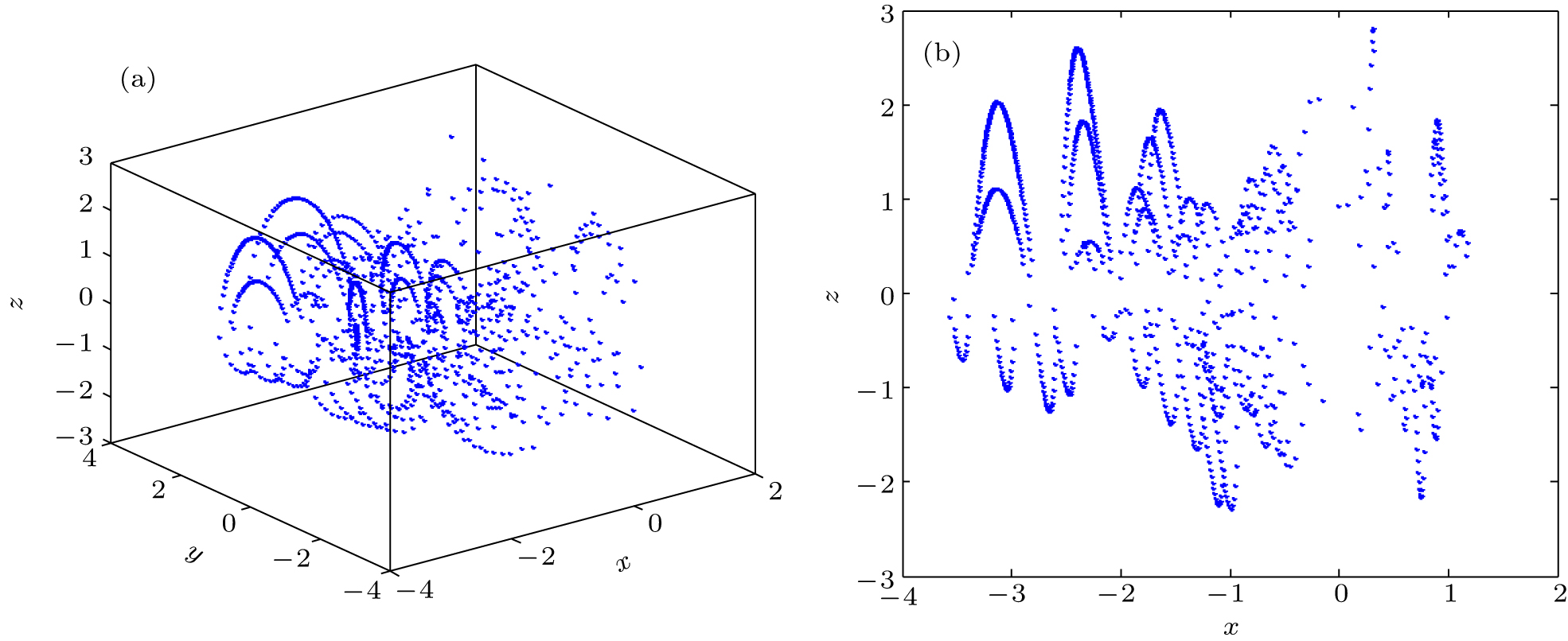 | Fig. 4. Poincare maps of the proposed fractional-order system without equilibrium points (16) when w = 0: (a) map in the 3D (x, y, z)-space; (b) map in the 2D (x, z)-plane. |
Referring to the power spectra, recall that chaotic dynamics is characterized by a continuous, broad-band and noise-like frequency spectrum. In particular, the frequency spectra of signals x(t) and w(t), numerically obtained from the proposed fractional-order hyperchaotic system (16), are shown in Figs. 5(a) and 5(b), respectively. As can be seen from Fig. 5, the spectra clearly show continuous and noise-like backgrounds, confirming that the fractional system (16) has a chaotic behavior.
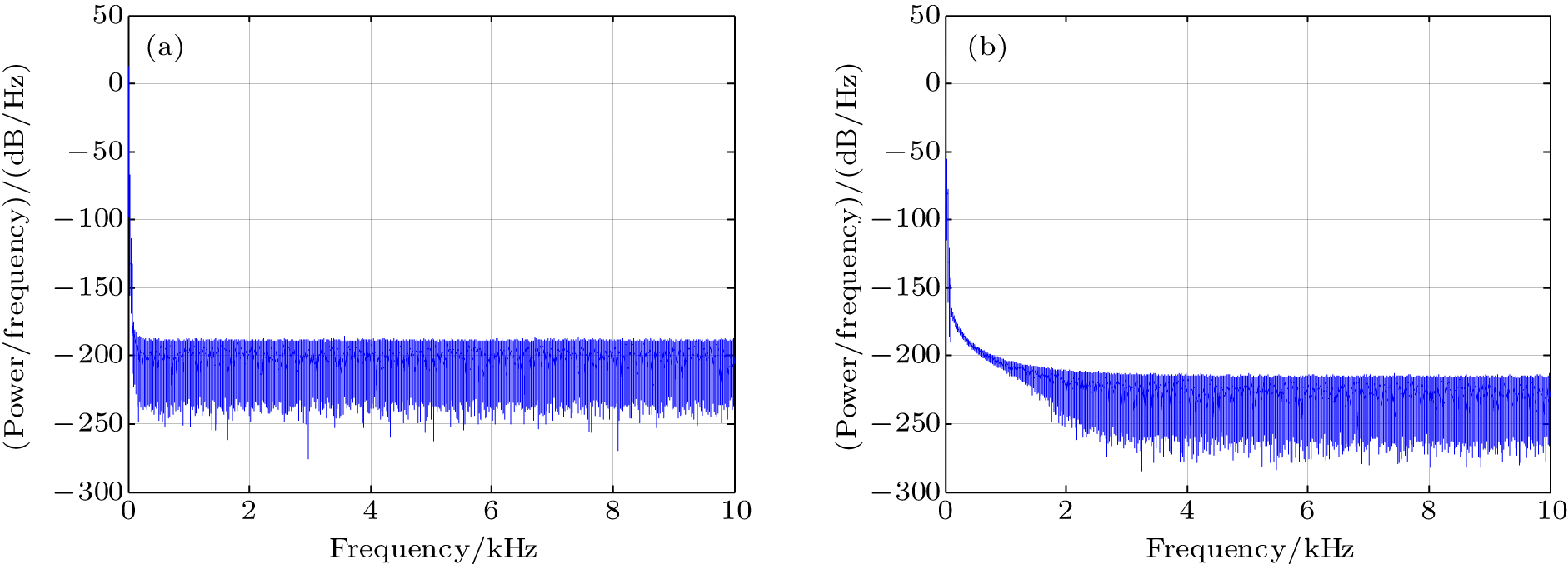 | Fig. 5. Frequency spectra obtained from the fractional-order system without equilibrium points (16): (a) hyperchaotic signal x(t); (b) hyperchaotic signal w(t). |
This Section is devoted to the study of the synchronization between hyperchaotic fractional-order systems.[39– 41] For this purpose, recall that the chaos synchronization between two dynamical systems (called drive and response systems, respectively) consists in making the state variables of the response system synchronized in time with the drive system states.[42– 48] A well-established technique to obtain synchronization is the observer-based method, where the response system is designed to behave as an observer of the drive system.[49, 50]
The aim of this section is to provide an example of observer-based synchronization applied to the hyperchaotic fractional-order system (16) with q = 0.96 and a = 8, b = − 2.5, and c = − 30. For this purpose, by exploiting the theoretical results developed in Refs. [49]– [51], the drive system can be written in the form of

whereas the synchronizing vector signal s(t) is

where K ∈ R3× 4 is a gain matrix to be determined.[50]
By using the synchronization method proposed in Refs. [49]– [51], the response system is
where ŝ (t) is the observer prediction of the synchronizing signal s(t), that is,

By defining the synchronization error between drive and response systems as

from Eqs. (20)– (23) it can be shown that the following linear fractional-order error system is obtained:

Now, it can be readily verified that the (4× 12)-controllability matrix derived from Eq. (25), i.e.,
is full rank. Therefore, according to Theorem 1 stated in Ref. [52], the eigenvalues of the error system (25) can be assigned anywhere in the stability region defined by the following inequality:

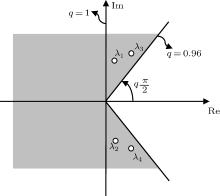
Note that the complex region of asymptotic stability, defined by inequality (27) for q = 0.96, is larger than the region corresponding to the integer-order case (the well-known open left half plane) since it includes a part of the right half plane shaped as a complementary wedge (Fig. 6). This distinctive property of fractional-order systems can be exploited in the considered hyperchaotic synchronization. For this purpose, the eigenvalues are selected to be (0.2 + i9.5, 0.2-i9.5, 0.5 + i10.04, 0.5 – i10.04), i.e., they have positive real parts but lie in the stability region depicted in Fig. 6.
 | Fig. 6. Stability region (in grey color) of the error system (25) under condition (27) for q = 0.96. The figure is not in scale. The selected eigenvalues (0.2 + i9.5, 0.2-i9.5, 0.5 + i10.04, 0.5 – i10.04) have positive real parts but belong to the stability region. |
Based on this choice, by using a standard Matlab® routine, the following feedback gain matrix is obtained:
which gives the linear error system
with eigenvalues(λ 1, λ 2, λ 3, λ 4) = (0.2 + i9.5, 0.2-i9.5, 0.5 + i10.04, 0.5-i10.04).
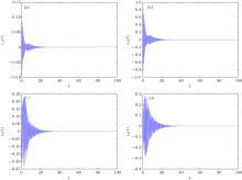
From Fig. 7, it can be observed that the fractional error system (29) is asymptotically stabilized at the origin (see inequality (27)), even though all the eigenvalues have positive real parts.
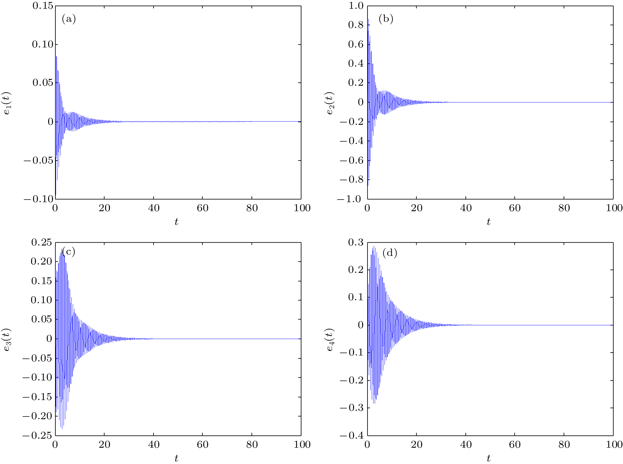 | Fig. 7. Time behaviors of the error system (29) for q = 0.96. |
Note that the plots reported in Fig. 7 are in agreement with the theoretical results expressed by condition (27) and proved in Ref. [52]. This indicates that the considered observer-based method enables hyperchaotic synchronization between the fractional drive system (20) and the fractional response system (22) to be effectively achieved.
The presence of hyperchaos in fractional-order systems without equilibrium points represents a new exciting phenomenon and an unexplored field of research. In this paper, this topic is investigated by introducing a new example of fractional-order hyperchaotic system without equilibrium. The considered approach uses the predictor-corrector algorithm to find the hyperchaotic attractor when the order of the derivative is q = 0.96. The considered fractional system is discussed, with the aim to further investigate its novel dynamical properties. Finally, an application of the observer-based synchronization to the proposed hyperchaotic fractional system is illustrated in detail.
| 1 |
|
| 2 |
|
| 3 |
|
| 4 |
|
| 5 |
|
| 6 |
|
| 7 |
|
| 8 |
|
| 9 |
|
| 10 |
|
| 11 |
|
| 12 |
|
| 13 |
|
| 14 |
|
| 15 |
|
| 16 |
|
| 17 |
|
| 18 |
|
| 19 |
|
| 20 |
|
| 21 |
|
| 22 |
|
| 23 |
|
| 24 |
|
| 25 |
|
| 26 |
|
| 27 |
|
| 28 |
|
| 29 |
|
| 30 |
|
| 31 |
|
| 32 |
|
| 33 |
|
| 34 |
|
| 35 |
|
| 36 |
|
| 37 |
|
| 38 |
|
| 39 |
|
| 40 |
|
| 41 |
|
| 42 |
|
| 43 |
|
| 44 |
|
| 45 |
|
| 46 |
|
| 47 |
|
| 48 |
|
| 49 |
|
| 50 |
|
| 51 |
|
| 52 |
|