


Inverse problem of quadratic time-dependent Hamiltonians
[Guo Guang-Jiea) , Meng Yana) , Chang Hongb) , Duan Hui-Zenga) , Di Bing†b)  ]
]
]


†Corresponding author. E-mail: dibing@hebtu.edu.cn
*Project supported by the National Natural Science Foundation of China (Grant No. 11347171), the Natural Science Foundation of Hebei Province of China (Grant No. A2012108003), and the Key Project of Educational Commission of Hebei Province of China (Grant No. ZD2014052).
Using an algebraic approach, it is possible to obtain the temporal evolution wave function for a Gaussian wave-packet obeying the quadratic time-dependent Hamiltonian (QTDH). However, in general, most of the practical cases are not exactly solvable, for we need general solutions of the Riccatti equations which are not generally known. We therefore bypass directly solving for the temporal evolution wave function, and study its inverse problem. We start with a particular evolution of the wave-packet, and get the required Hamiltonian by using the inverse method. The inverse approach opens up a new way to find new exact solutions to the QTDH. Some typical examples are studied in detail. For a specific time-dependent periodic harmonic oscillator, the Berry phase is obtained exactly.
The harmonic oscillator[1] is an extremely important model in quantum mechanics and leads to many important insights. In addition, when we consider systems that have interactions with changing surroundings, it is convenient to introduce the time-dependent Hamiltonian to provide a phenomenological description. The Paul trap[2] is just one example of time-dependent harmonic oscillators (TDHO), in which the frequency is time-dependent. TDHO have many applications in many branches of physics, including molecular physics, quantum chemistry, and quantum optics.[3– 7] However, the TDHO are among only a very few exactly solved time-dependent systems, [8– 10] although many approaches have been used. The quantum-invariant method was invented by Lewis and Riesenfeld[11, 12] to solve the TDHO Hamiltonian, and in the following decades, many other analytical methods were discovered, such as the orthogonal functions invariant method, [13, 14] the algebraic method, [15, 16] the evolution operator method, [17] and the propagator method[18] among others. Based on the analytical solutions of the time-dependent periodic harmonic oscillator, the Berry phase can be obtained if the solutions are stable.[19, 20]
In distinction from the harmonic oscillator, the inverse harmonic oscillator (IHO) has a continuous spectrum and is doubly degenerate.[21] The IHO also has many applications in various fields, such as in studies of the expansion of the early universe and the study of black holes, [22, 23] open quantum systems, [24– 26] nuclear fission, [27] and reactive scattering.[28] It may serve as a test and illustration of various approximation methods.[29– 31] Therefore, it is also worth making the effort to obtain the solutions of the time-dependent inverse harmonic oscillator (TDIHO). Since both the TDHO and TDIHO possess the same SU(1, 1) algebraic structure, many methods of solving TDHO problems are also applicable in the TDIHO problem. Hence for as long as we focus only on the methodology, it is not necessary to make a distinction between the TDHO and TDIHO, both of which will be referred to as quadratic time-dependent Hamiltonians (QTDH). However, a huge difference arises once one investigates the properties of solutions of the TDHO and TDIHO. Using the invariant method of Lewis and Riesenfeld, the exact wave function of the TDIHO has been obtained in terms of the Weber function.[32– 34] With the evolution operator method, the quantum tunneling effect of the coherent states and the Gaussian wave-packet in the inverse Caldirola– Kanai harmonic oscillator have been studied at length.[35– 37] Recently, we proposed an algebraic method[38] to obtain the temporal evolution wave function of the Gaussian wave-packet in the TDIHO. In particular, the quantum tunneling effect and the sojourn time of the Gaussian wave-packet were studied.[38] On the basis of this algebraic method, the counterintuitive properties of the sojourn time of the IHO on the two-dimensional (2D) noncommutative plane were discussed in Ref. [39]. In addition, the temporal evolution of the TDIHO in arbitrary dimensions has also been investigated.[40]
Many studies have shown that in order to solve a QTDH problem a key step is to get the general solution of a Riccatti equation or its deformation. However, the Riccatti equation is a nonlinear differential equation and the known analytic solutions are limited. Therefore, most practical cases are generally unsolvable in exact expressions. On the other hand, we often wish to obtain a wave-packet with a particular evolution. We then need to know the QTDH required to get this evolution. We call this problem the inverse QTDH problem. It is interesting that getting the Hamiltonian that yields a specific evolution is much easier than solving the Schrö dinger equation with a given Hamiltonian. This reverse idea is also very useful for discovering many new exact solutions to the QTDH. In addition, for some specific periodic Hamiltonians it is also possible to find their exact Berry phase.
The paper is organized as follows: in Section 2, the formal solution of the wave-packet’ s evolution wave function is obtained using the algebraic method. This is within the context of the direct QTDH problem. In Section 3, the inverse problem method for the QTDH is developed. Some typical examples are calculated in Section 4. For a specific time-dependent periodic harmonic oscillator, the Berry phase is obtained exactly in Section 5. A brief summary and remarks are presented in Section 6.
The quadratic time-dependent Hamiltonian can be written as

where p̂ and x̂ are operators of the momentum and coordinate respectively, and 


It is easy to show that the Hamiltonian (1) has an SU(1, 1) algebraic structure, whose generators satisfy the relations

with the following realization

The time-dependent Schrö dinger equation is

The Hamiltonian (1) can be simplified by an appropriate unitary transformation given by

where v_(t) and v0(t) must satisfy the conditions

The dots on the top of functions denote differentiation with respect to t. The second differential equation in Eq. (6) is a Riccatti equation, and for an arbitrary 
The transformed Hamiltonian then becomes

Now, it is easy to obtain the solution of the time-dependent Schrö dinger equation with the transformed Hamiltonian (7)

where |p〉 is the eigenstate of momentum p̂ with eigenvalue p which can be an arbitrary real number. The phase function θ p(t) is given by
We can then obtain the solution of the time-dependent Schrö dinger equation with the original Hamiltonian (1)

Choosing the initial condition v0(0) = v_(0) = 0, this solution describes the temporal evolution of the plane wave |p〉 . Therefore, the temporal evolution of an arbitrary initial state

can be expressed as

We consider the temporal evolution of a minimum-uncertainty wave-packet stationed initially at the origin, and written as

After a Fourier transformation, equation (13) can be expressed in momentum representation, as

Substituting Eqs. (10) and (14) into Eq. (12), one can obtain the temporal evolution wave function as

where we have used the notations
Thus, at any time the probability density distribution of the particle is always Gaussian, and is given by
However, the width Δ x2(t) of the wave-packet is time-dependent with
So far the problem of the wave-packet’ s evolution in QTDH has been solved formally, but in practical cases one must obtain the exact solution of Eq. (5), which may be difficult because the second differential equation in Eq. (6) is a Riccatti equation. This is a nonlinear differential equation for which the known analytic solutions are very limited.
On the other hand, if one wishes to deal with a wave-packet with a particular known evolution, then the problem becomes that of finding the Hamiltonian required to yield this temporal evolution. We call this problem the inverse QTDH problem. One of the important physical quantities of the wave-packet is its width. Therefore, in the following we start with the desired temporal evolution function of the wave-packet’ s width, and deduce the required Hamiltonian. We will see that solving the inverse problem is much easier than the direct problem. Our analysis will greatly enrich the number of known analytical solutions to the QTDH.
Since we start with the wave-packet’ s width, we will adopt an appropriate unit. Without loss of generality, we set the initial value of the wave-packet’ s width as one unit, i.e., λ 0 = 1. Thus, the new units of length and time become 
According to Eq. (16), we can obtain

Thus, equation (19) can be rewritten as
It can be easily verified that the above equation can be expressed as

where the constant C will be determined by the initial condition, and we have introduced an assistant function F(t), defined as

According to the initial condition v0(0) = v_(0) = 0 and Eq. (16), we have A(0) = 0. Thus from Eq. (22) we obtain C = − F(0). Therefore, equation (22) can be rewritten as

We take the derivative on both sides of Eq. (24), and have

where

Hence, one can obtain the relation between v0(t) and the wave-packet’ s width Δ x2(t), as

On the other hand, from equation set (6) one can obtain the differential equation satisfied by v0(t) as

Substituting Eq. (27) into the above equation, one can obtain a surprisingly simple expression relating 

where f(t) is defined in Eq. (26). The validity of Eq. (29) can be confirmed for the free particle case, the harmonic oscillator and the inverse harmonic oscillator case, respectively. The evolution functions of the wave-packet width in the free particle case, the harmonic oscillator case, and the inverse harmonic oscillator case are (1 + t2)/2, 1/2, and (cosh2t)/2, respectively. Substituting them into Eq. (29), one obtains 


In addition, if the initial center of the wave-packet is not at the origin (i.e., x0 ≠ 0), then we have the temporal evolution of the wave-packet’ s center as derived in Ref. [38], and given by

Substituting Eq. (27) into the above equation, we obtain the evolution function of the center of the wave-packet as
By analyzing the evolution function of the center of the wave-packet one can deduce the stability of the system.[2]
We suppose that the evolution function of the wave-packet width obeys power law diffusion:

The case b = 2 corresponds to the free wave-packet, i.e., 

According to Eq. (31), the evolution function of the wave-packet’ s center can be shown to be

where F(α , β , γ , z) is the hypergeometric function.[41]
We now suppose that the evolution function of the wave-packet width obeys power law compression:

Substituting Eqs. (26) and (35) into Eq. (29), we obtain

According to Eq. (31), the evolution function of the wave-packet’ s center can be shown to be

From the expression (37), one can easily see that in this case the vibration frequency of the wave-packet center increases as time increases, but the vibration amplitude of the wave-packet center is compressed as time increases.
Finally, we consider the case where the evolution function of the wave-packet width obeys spiral exponent diffusion:

Substituting Eqs. (26) and (38) into Eq. (29), we have
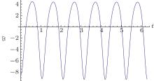
From the above expression, we can obtain that as t increases the potential will gradually become periodic. Figure 1 shows the function 
 | Fig. 1. Diagram of the required  |
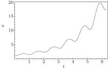
Moreover, according to Eq. (31) the evolution function of the wave-packet center can be found to have the form shown in Fig. 2.
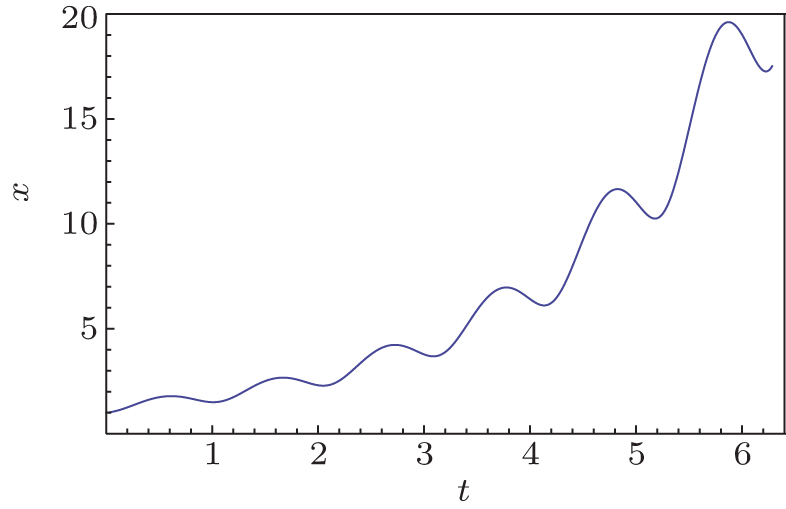 | Fig. 2. Diagram of x(t) when Δ x2(t) obeys spiral exponent diffusion. Here we take ω = 3, σ = 1. |
In this section, we consider the case where the evolution function of the wave-packet’ s width is periodic, and obtain the required Hamiltonian. In addition, the Berry phase of the temporal evolution of the wave-packet is investigated. First, we suppose that the desired evolution function of the wave-packet’ s width is:

Its period is π /ω .
Substituting Eqs. (26) and (40) into Eq. (29), we obtain

One can easily show that this potential is periodic and that the period is also π /ω . Figure 3 shows 
 | Fig. 3. Diagram of the required  |
Hence, the required Hamiltonian can be written as

According to Eq. (31), the evolution function of the wave-packet center can be written as

Figure 4 is a diagram of the wave-packet center showing the periodic oscillation. From this figure and Eq. (43) we can easily see that the position of the center of the wave-packet moves periodically with period π /ω .
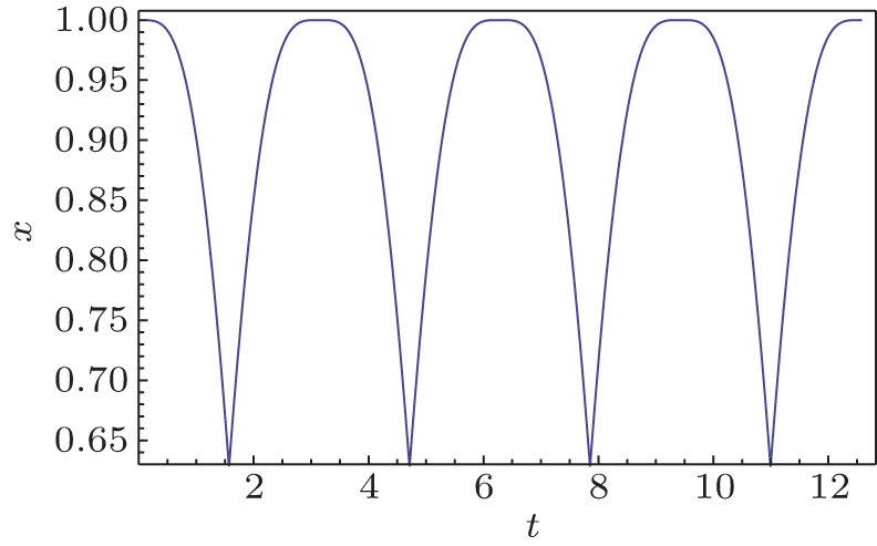 | Fig. 4. Diagram of x(t) when Δ x2(t) is the periodic function of Eq. (40). Here we take ω = 1. |
In the following, we obtain the exact analytical temporal evolution wave function of the wave-packet. The Berry phase of the wave-packet can then also be investigated. From Eq. (15), we know that the wave function of the wave-packet is determined by three functions: A(t), χ (t), and v_(t). According to Eqs. (23), (26), and (40), one can easily obtain

The expressions for A(t), χ (t), and v0(t) can be obtained using Eqs. (20), (24), and (27). Moreover, the expression of v_(t) can be obtained by using v0(t) and Eq. (6). Thus, we have
Finally, substituting Eq. (45) into Eq. (15), one can obtain the exact analytical temporal evolution wave function of the wave-packet. It is worth noting that the functions A(t), χ (t), and v_(t) are all periodic, and that the periods are all π /ω . Therefore, we have

where the overall phase change is

On the other hand, during the first period, π /ω , of the evolution, the dynamical phase change is δ d given by

Berry’ s phase δ B is obtained from the overall phase by subtracting the dynamic phase:

Since Ψ (x, t) satisfies the Schrö dinger equation (4), equation (49) can be rewritten as

Considering this case, the Hamiltonian 


Therefore, Berry’ s phase is described as a one loop integral in the parameter space.[42]
Using Eqs. (15), (42), (45), and (49), we obtain the expression for Berry’ s phase δ B in the form
It is difficult to evaluate the integral on the right-hand side of Eq. (52) analytically. However, one can obtain the analytical results for some limiting cases. First, let us consider the high frequency range, i.e., ω ≫ 1. In this limit, the integrand on the right-hand side of Eq. (52) can be written as

Thus, Berry’ s phase is given exactly by
We thus obtain that the Berry’ s phase and frequency ω are linearly related in high frequency. On the other hand, for ω ≪ 1 Berry’ s phase is ill-posed, and is not considered.
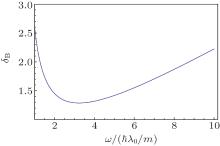
For finite ω the integral in Eq. (52) can be calculated numerically and the relation between Berry’ s phase and frequency ω can be obtained. The numerical result in Fig. 5 shows that for finite ω the Berry’ s phase is a concave function of ω and has a minimum at ω ≈ 3.2257. Since the unit of ω is ħ λ 0/m, the initial value of the wave-packet’ s width also influences Berry’ s phase through this unit.
 | Fig. 5. Plot of Berry’ s phase δ B: Berry’ s phase is a concave function of ω and has a minimum at ω ≈ 3.2257. The unit of ω is ħ λ 0/m. |
Let us summarize our results as follows. The formal solution for the wave-packet evolution wave function is obtained for the QTDH by using the algebraic method. However, most practical cases are generally not exactly solvable since we need the general solution of the Riccatti equations. We have therefore chosen to address the inverse problem. We start with a specific temporal evolution function for the wave-packet width, and using the inverse method developed in Section 3 obtain the QTDH. It turns out that getting the Hamiltonian corresponding to a given solution is much easier than solving the Schrö dinger equation for a given Hamiltonian. As is well known, analytical solutions to QTDHs are invaluable in many areas of physics, and our inverse approach opens up a new way of finding novel exact solutions to QTDH. As some typical examples, we obtained the exact QTDH expressions for cases where the evolution function of the wave-packet’ s width obeys power law diffusion, power law compression, and spiral exponent diffusion. For the case of a periodic oscillation, we obtained the Hamiltonian and the exact wave function of the wave-packet. In this periodic Hamiltonian system, the Berry phase of the wave-packet can be obtained directly. The results show that in our specific periodic Hamiltonian (42) the Berry phase and frequency ω are in a linear relationship for high frequencies. In addition, we have calculated the Berry phase numerically for finite ω . The numerical result shows that for finite ω the Berry phase is a concave function of ω . Since the units of ω contain the initial wave-packet’ s width, the initial value of the wave-packet’ s width can influence the Berry phase.
| 1 |
|
| 2 |
|
| 3 |
|
| 4 |
|
| 5 |
|
| 6 |
|
| 7 |
|
| 8 |
|
| 9 |
|
| 10 |
|
| 11 |
|
| 12 |
|
| 13 |
|
| 14 |
|
| 15 |
|
| 16 |
|
| 17 |
|
| 18 |
|
| 19 |
|
| 20 |
|
| 21 |
|
| 22 |
|
| 23 |
|
| 24 |
|
| 25 |
|
| 26 |
|
| 27 |
|
| 28 |
|
| 29 |
|
| 30 |
|
| 31 |
|
| 32 |
|
| 33 |
|
| 34 |
|
| 35 |
|
| 36 |
|
| 37 |
|
| 38 |
|
| 39 |
|
| 40 |
|
| 41 |
|
| 42 |
|