


Fractional-order Lβ Cα filter circuit network
[Hong Zhenga) , Qian Jing†a)  , Chen Di-Yi
b) , Herbert H. C.Iuc) ]
, Chen Di-Yi|
|


†Corresponding author. E-mail: qianjingkg@163.com
*Project supported by the National Natural Science Foundation of China (Grant No. 51469011).
In this paper we introduce the new fundamentals of the conventional LC filter circuit network in the fractional domain. First, we derive the general formulae of the impedances for the conventional and fractional-order filter circuit network. Based on this, the impedance characteristics and phase characteristics with respect to the system variables of the filter circuit network are studied in detail, which shows the greater flexibility of the fractional-order filter circuit network in design. Moreover, from the point of view of the filtering property, we systematically study the effects of the filter units and fractional orders on the amplitude–frequency characteristics and phase–frequency characteristics. In addition, numerical tables of the cut-off frequency are presented. Finally, two typical examples are presented to promote the industrial applications of the fractional-order filter circuit network. Numerical simulations are presented to verify the theoretical results introduced in this paper.
The analysis and modeling of large LC filter circuit networks has drawn a great deal of interest from all natural sciences, since the beginning of the 20th century.[1, 2] At present, the LC filter circuit is an important passive filter circuit due to its better filtering properties and simple structure. Over the past few decades, researchers have published lots of papers on the LC filter circuit.[3– 6] The topic becomes even popular when Andre Geim and Konstantin Novoselov won the 2010 Nobel Prize in Physics for their investigations of the resistance networks of graphene. The circuit network is more coincident with the natural attributes of the material world, and it has better properties in engineering applications than the simple circuit unit.[7– 10] Therefore, we focus on LC filter circuit networks. However, fewer scientists have attempted to broaden the scope of fundamentals and theorems from integer order systems into fractional ones, [11, 12] although the applications of fractional calculus have many advantages, such as more flexibility, freedom, best fit, and optimization techniques.
Fractional calculus has been attracting more and more researchers from science to engineering.[13– 16] Fractional calculus can be considered as a super set of integer-order calculus, which has the potential to accomplish what the integer-order cannot realize because of the existence of an extra degree of freedom.[17, 18] Since fractional calculus depends on the history of the function, it is more suitable and realistic for applications such as designing novel modulation schemes in communications, signal progressing, system identification, controlling, and mathematical modeling.[19– 23] More specifically, some researchers have been devoting their efforts on the design and realization of the fractional electronic components.[24– 27] Motivated by the above analysis, circuit designers will have to face new challenges to the new phenomenon and laws due to the applications of the fractional-order components.
From the above considerations, new laws and fundamentals of the fractional-order filter circuit network are mainly studied, for which there are four traditional variables: L, C plus two fractional orders α and β . Therefore, there should appear interesting phenomena in the fractional-order filter circuit network, which cannot be obtained in the conventional filter circuit networks.
The following advanced research contents can make our research attractive. First, the new fundamentals of the impedance and phase characteristics are systematically studied, which lays the groundwork for the design of the fractional-order filter circuit network. Second, from the point of view of the circuit, as a new concept, the inductance value power loss is presented in view of the energy loss. Furthermore, the amplitude– frequency characteristics, phase– frequency characteristics, and cut-off frequency are studied in detail with respect to the number of filter units and the fractional orders. Finally, two application cases are presented to show the better filter properties of the fractional-order filter circuit network.
The rest of this paper is organized as follows. In Section 2 the fundamentals of the conventional filter circuit networks are analyzed. In Section 3, basic definitions of fractional-order capacitors and inductors are presented, and the new fundamentals of the fractional-order filter circuit network are discussed, including the impedance characteristics, phase characteristics, amplitude– frequency characteristics, phase– frequency characteristics, and cut-off frequency. Two typical examples about applications are presented in Section 4. In Section 5 some conclusions are drawn from the present study.
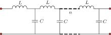
The conventional LC filter circuit network is presented in Fig. 1. From Fig. 1, with a unit, the Laplace transform expression of the impedance can be given by

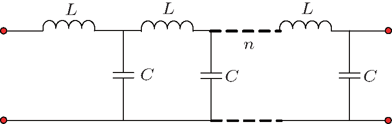 | Fig. 1. Diagram of the conventional LC filter circuit network. |
With two units in the filter circuit, the impedance is also expressed as
Similarly, when there are three units in the filter circuit, one has
From Eqs. (1), (2), and (3), when there are infinite units in the filter circuit network, we can obtain the impedance as

Furthermore, one obtains

Thus, from Eq. (5), the impedance can be rewritten as

Hence, its magnitude of the impedance of the filter circuit network can be expressed as
Moreover, from Eq. (6), the phase of the conventional filter circuit network can be expressed as
From Eq. (7), the large impedance value will be obtained with larger L or smaller C. However, there is no relation between the impedance and the frequency, which validates the deficiency of the conventional filter circuit network in design.
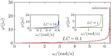
Figure 2 shows the phase response of the conventional filter circuit network for different values of LC, where the phase increases with the increase of the frequency. Clearly, a critical minimum exists when ω 2LC tends to 4, and its location changes as LC changes. Moreover, its frequency range is too narrow, which restricts the potential for circuit design and control, and reduces its applications.
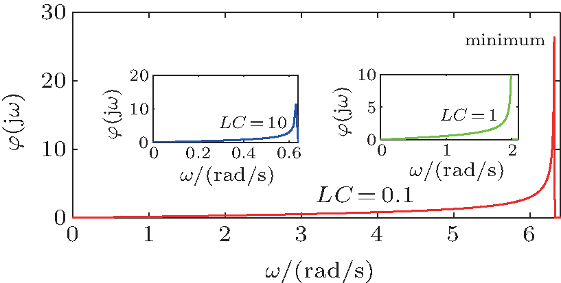 | Fig. 2. Phase response of conventional filter circuit network for different LC values. |
At present, there are three frequently-used definitions of the fractional derivative, which are the Grunwald– Letnikov, the Riemann– Liouville, and Caputo definitions.[28] Here, we use the Caputo definition of the fractional derivative over other definitions because the initial conditions of this definition take the same form as the more familiar integer-order differential equations. The fractional derivative by Caputo is denoted as
where Γ (x) is the well-known Euler’ s Gamma function and n − 1 ≤ α ≤ n.
Under zero initial conditions, we apply the Laplace transform to the Caputo definition (9). Thus, one obtains

Furthermore, we use the relationship between the voltage and current of the fractional-order capacitors and inductors. Consequently, the following expressions can be obtained:

and

Similarly, under zero initial conditions, by applying the Laplace transform to Eqs. (11) and (12), the impedances of the fractional-order capacitors and inductors can be rewritten as 

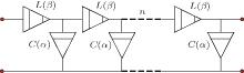
The diagram of the fractional-order filter circuit network is shown in Fig. 3. Therefore, its impedance can be derived as
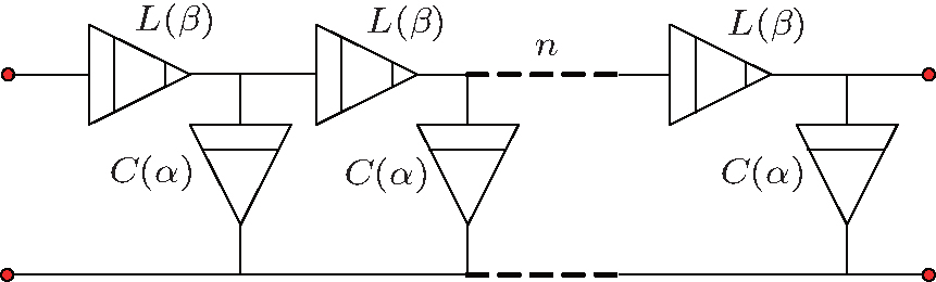 | Fig. 3. Diagram of the fractional-order LC filter circuit network. |
The equivalent impedance of the fractional-order filter circuit network is shown in Eq. (13). Note that two extra variables, the fractional orders α and β , are included in the impedance. Moreover, the impedance varies with the five parameters, i.e., L, C, the frequency ω , the fractional-orders α and β . For the conventional case, the previous conditions cannot be satisfied.
Therefore, the new laws and fundamentals of the fractional-order filter circuit network will be systematically studied in the following subsections.
In this subsection, we study the impedance characteristics of the fractional-order filter circuit network in detail.
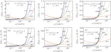
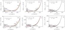
Figure 4 shows the relations between the impedance value and the fractional β for different values of L and C. It is clear from Fig. 4 that the impedance values decrease with the increase of β in low frequency region (ω < 1). However, it is quite the opposite in high frequency region (ω > 1). Interestingly, there is an intersection point for all curves with ω tending to 1, which can be explained by that ω β , ω 2β , and ω β − α play the leading role in Eq. (13).
 | Fig. 4. Absolute values of the impedance vary with the frequency of fractional-order filter circuit network with different values of fractional order β for C = 1 (a), 10 (b) and 100 (c) and L = 1 (d), 10 (e), and 100 (f). |
Comparing Figs. 4(a)– 4(c), with the increase of C, the impedance decreases, which means that the inductance value power loss can be reduced, especially in the large or medium power applications. Such interesting phenomena can be explained by the dominant role of 
Also, the impedance results in Figs. 4(d)– 4(f) agree with the expected outcomes, in that the impedance increases as L increases. It is mainly due to the notable positive correlation between the impedance and L in Eq. (13).
Given all that, it is worth noting that the smaller inductance value power loss can be obtained with the larger fractional order β , the smaller L, and the larger C in the fractional-order filter circuit network. More significantly, the smaller L can effectively reduce the volume of the filters from the viewpoint of engineering.
Figure 5 presents the relations between the impedance value and the fractional α for different L and C values. From Fig. 5, the impedance increases gradually with the increase of α in the low frequency region. Moreover, with the increases of L and C values, the curves are merged into a line in the high frequency region. In other words, the effect of fractional order α on the impedance is very small in the high frequency region when L and C values are large.
As expected, it is clear from Figs. 5(a)– 5(c) that the inductance value power losses decrease with the increase of C, which are consistent with the impedance results in Fig. 4.
Similarly, with the increases of L values in Figs. 5(d)– 5(f), the inductance value power losses increase.
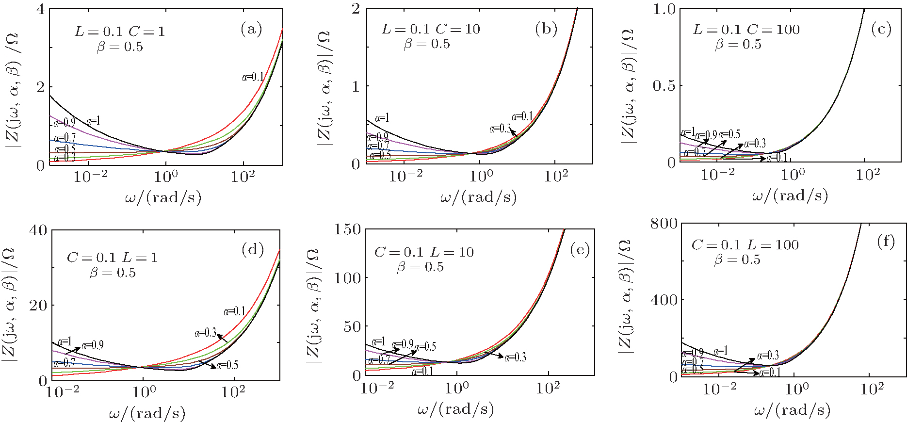 | Fig. 5. The absolute value of the impedance varies with the frequency of the fractional-order filter circuit network with different values of fractional order α for C = 1 (a), 10 (b), and 100 (c) and L = 1 (d), 10 (e), and 100 (f). |
Note that we can obtain the smaller inductance value power loss with the smaller fractional order α , smaller L, and larger C, which is a meaningful conclusion in engineering practice.
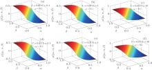
The graphic model is presented in Fig. 6 to describe the relationship between the impedance and the fractional orders with different L and C values.
 | Fig. 6. Graphic model of the absolute value of the impedance for fractional-order filter circuit networks with C = 1 (a), 10 (b), and 100 (c), L = 1 (d), 10 (e), and 100 (f). |
From Fig. 6, the inductance value power losses gradually decrease with the increase of β and the decrease of α . In addition, the impedance decreases with the increase of C, while the impedance increases with the increase of L. Such results are consistent with the above analyses. Therefore, whether the effect of the fractional orders can increase or decrease depends on the requirement of the application.
In this subsection, the phase diagrams of fractional-order filter circuit networks are presented to describe the phase characteristics in detail.
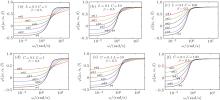
The relations between the phase response and the frequency with different values of fractional order β for different L and C values are shown in Fig. 7. Clearly, with the increase of frequency, all curves reach different maximal values. Specifically, the effect of frequency on phase is small for each curve in low and high frequency regions. Moreover, the phase increases as the fractional-order β increases, with frequency fixed. Interestingly, the phase value is maintained at zero with the smaller L and C values in the low frequency region when α = β = 0.5, which is a meaningful conclusion.
 | Fig. 7. Phase responses of the fractional-order filter circuit network vary with the frequency with different fractional-order β for C = 1 (a), 10 (b), 100 (c), L = 1 (d), 10 (e), and 100 (f). |
Comparing the panels in the figure, the phase increases with the increases of L and C values, which means the fixed maximal phase values can be obtained at the lower frequency with the increases of L and C values. However, it is worth noting that the fixed maximal phase value is not affected by L and C.
Figure 8 illustrates relations between the phase response and the frequency with different values of fractional-order α for different L and C values. It is clear from these panels that all curves reach the same maximal phase value with the increase of frequency. Comparing the curves in the panels, the phase decreases as α increases in the low frequency region. In addition, the increasing rate of the phase increases with the increase of the fractional-order α , which means that the fixed maximal phase can be obtained at the lower frequency with larger α .
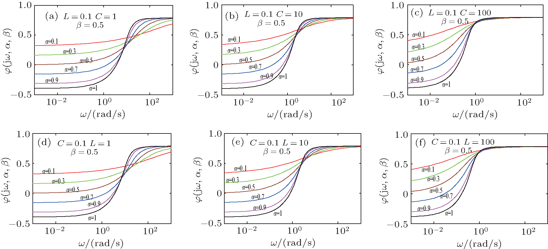 | Fig. 8. Variations of phase responses of the fractional-order filter circuit networks with the frequency with the different values of fractional order α for C = 1 (a), 10 (b), 100 (c), L = 1 (d), 10 (e), and 100 (f). |
Comparing the panels in Fig. 8, with the increases of L and C values, the phase gradually increases. In other words, the fixed maximal phase can be obtained at the lower frequency with larger L and C values. However, the effects of L and C on the fixed maximal phase are very small. Moreover, the effects of the fractional-order α on the phase response can be reduced at the high frequency when L and C values are larger.
The graphic models are presented in Fig. 9 to describe the relations between the phase response and the fractional order with different L and C values.
 | Fig. 9. Graphic model of the phase response versus fractional orders α and β of the fractional-order filter circuit networks with C = 0.1 (a), 1 (b), 10 (c), L = 0.1 (d), 1 (e), and 10 (f). |
From Fig. 9, the larger phase value of the fractional-order filter network can be obtained with smaller α and larger β , which are consistent with the above analyses. Meaningfully, the zero phase can also be obtained when α = β = 0.5, which means that the filter circuit network can not only keep the lag of the phase, but also keep the leading phase.
It should be noted that there are some critical values and special cases with the fractional-order capacitors and inductors used in the filter circuit network; such a finding can be ascribed to the existence of the fractional orders, which reflects the greater flexibility of the fractional-order filter circuit network in circuit design.
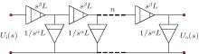
The diagram of the fractional-order filter circuit network is shown in Fig. 10. When there are infinite elements of the filter unit, the operational amplifiers are omitted because of the accumulative effects of loads.
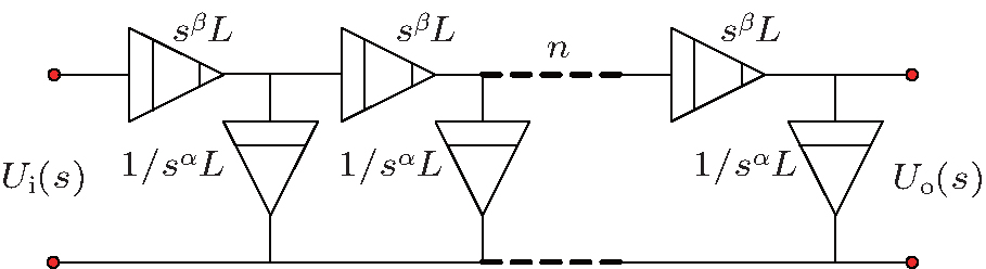 | Fig. 10. Diagram of the fractional-order filter circuit network with n filter units. |
From Fig. 10, the voltage gain function is presented as

where n is the number of the filter units.
Therefore, the expression of the frequency characteristic is easily given according to the relationship between the frequency characteristic and the voltage gain function as

where n is the number of filter units.
The amplitude– frequency characteristic is an important reflection of the filtering properties. Therefore, in this subsection, we systematically analyze the amplitude– frequency characteristics of the fractional-order filter circuit network varying with the fractional order, α + β and the number of filter units.
Figure 11 illustrates the relations between the magnitude response of Eq. (15) and f for different numbers of filter units. From Fig. 11, the following new amplitude– frequency characteristics of the fractional-order filter circuit network can be obtained.
 | Fig. 11. Amplitude– frequency characteristics of the fractional-order filter circuit network versus the number of filter units when LC = 10 and α + β = 1.5. |
Ripple output: the ripple output becomes large with the increase of the number of filter units.
Passband gain: the fractional-order filter circuit network will obtain higher passband gain with more filter units in the passing band of the fractional-order filter circuit network, which means that the preferable effect of the passband gain can be acquired with fewer filter units.
Bandwidth and filter factor: the bandwidth and the filter factor of the fractional-order filter circuit network are smaller and smaller with the increase of filter units, which indicates the filter circuit can obtain better frequency resolution and selectivity.
Damping coefficient and quality factor: the inductance value power loss is less at a fixed frequency with more filter units due to the smaller damping coefficient. However, the quality factor is quite the opposite according to the relationships between the damping coefficient and the quality factor.
The cut-off frequency, whose alias is half the power frequency, can be obtained by solving the following equation

The effects of the number of filter units are shown in Table 1.
| Table 1. Cut-off frequencies of the fractional-order filter circuit network with LC = 10, α + β = 1.5 for different numbers of filter units n. |
With the increase of the number of filter units, the cut-off frequency gradually decreases when n < 8 (see Table 1). However, the effect of the number of filter units on the cut-off frequency is very small when n > 8. Therefore, the minimal effect of the number of filter units on cut-off frequency can be obtained when n > 8.
The relations between the amplitude– frequency characteristics and the fractional order are presented in Fig. 12. From Fig. 12, the ripple output, passband gain, and selectivity of the octave of the fractional-order filter circuit network are better than those of the conventional filter circuit network when α + β = 4. In summary, the fractional-order filter circuit network can obtain better filtering properties.
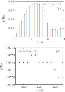
Similarly, the cut-off frequencies calculated with fixed LC and n for different fractional-orders α + β are shown in Fig. 13.
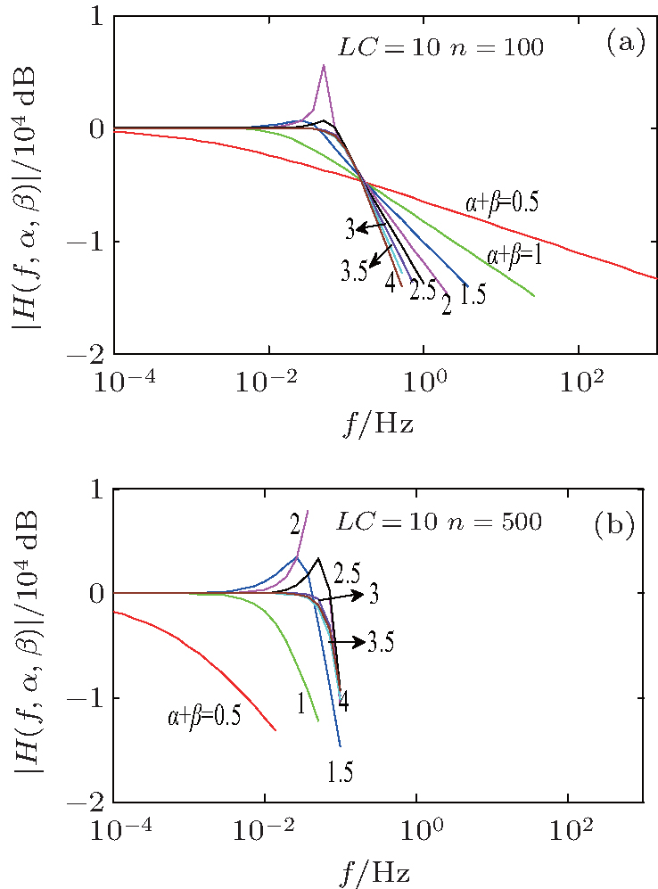 | Fig. 12. Amplitude– frequency characteristics of the fractional-order filter circuit network versus the fractional-order α + β when LC = 10, n = 100 (a) and 500 (b). |
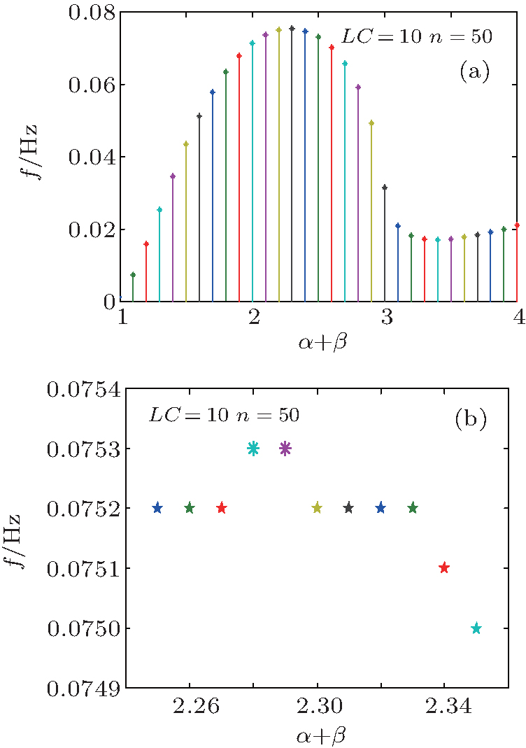 | Fig. 13. Cut-off freqencies of the fractional-order filter circuit network versus fractional-order α + β when LC = 10 and n = 50. |
From Fig. 13(a), the cut-off frequency increases rapidly first and then decreases, and then increases slowly with the increase of the fractional-order α + β . In other words, there is a great effect of the filter units on the cut-off frequency. From Fig. 13(b), it is clear that there is a critical cut-off frequency when α + β = 2.28 or α + β = 2.29.
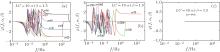
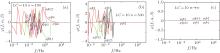
The phase– frequency characteristics are also an important indicator of the filtering properties, and the system analysis is the main part of the subsection. Furthermore, the relations between the phase– frequency characteristics of the fractional-order filter circuit network and fractional-orders α + β and the number of filter units are analyzed below.
Figure 14 shows the phase– frequency characteristics for different numbers of filter units. From Fig. 14, the phase value tends to be stable at lower frequency with the increase of the number of filter units n for a certain fractional order, α + β . In addition, the phase value is equal to zero as the number of filter units n tends to infinity. In this case, there is, however, no value in the low frequency region. In a purely mathematical sense, this is obviously due to the fact that there is no result in seeking answers to the phase in Eq. (10).
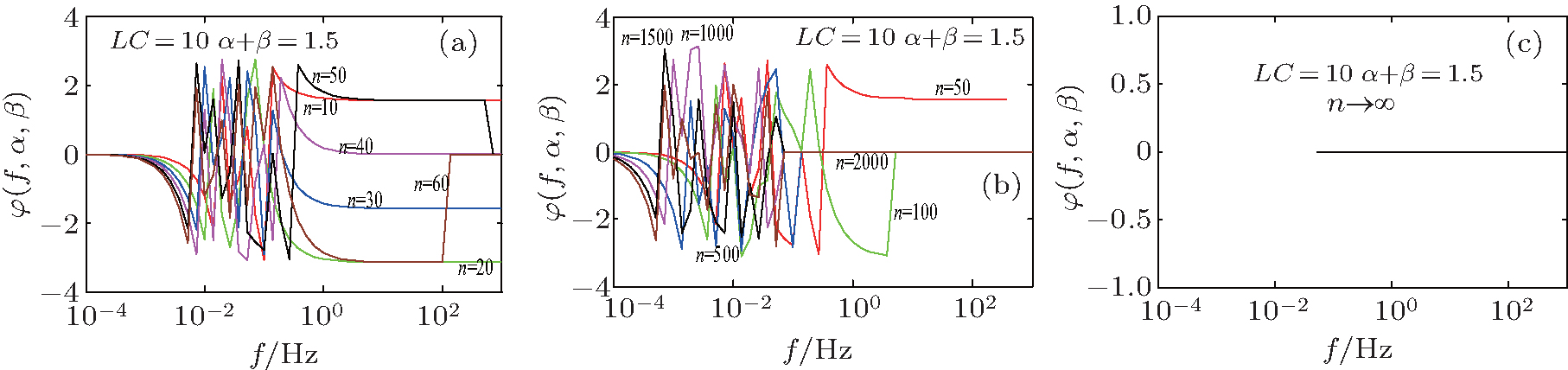 | Fig. 14. Phase– frequency characteristics of the fractional-order filter circuit network for different numbers of filter units when LC = 10 and α + β = 1.5. |
Figure 15 shows the plots of phase– frequency characteristics versus frequency for different fractional orders. With the increase of the frequency in Fig. 15, all curves gradually reach zero phase with a certain number of filter units. Furthermore, when the number of filter units tends to infinity, it should be noted that the phase value is equal to zero, which indicates the filter circuit keeps not only the lagging phase, but also the leading phase in the passing band.
 | Fig. 15. Phase– frequency characteristics of the fractional-order filter circuit network for different values of fractional-order α + β when LC = 10 and n tends to infinity in steps. |
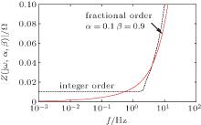
The inductance value power loss for the fractional-order filter circuit network is almost an inevitable consequence because of the existence of the inductance. Consequently, the inductance value power loss does not merely increase the power waste of the fractional-order filter circuit network, but also it has an adverse effect on the filter. Therefore, it is meaningful to reduce the inductance value power loss under the given conditions.
The relations between the impedance and the frequency of the conventional and fractional-order filter circuit network are illustrated in Fig. 16. Comparing the curves, we can clearly observe that the impedances of the fractional-order filter circuit networks with certain fractional orders are smaller than those of the conventional filter circuit networks except for a part of the frequency region, which means the inductance value power loss can be reduced in the fractional-order filter circuit network. Considering the energy loss, the application of the fractional-order filter circuit network is of practical significance.
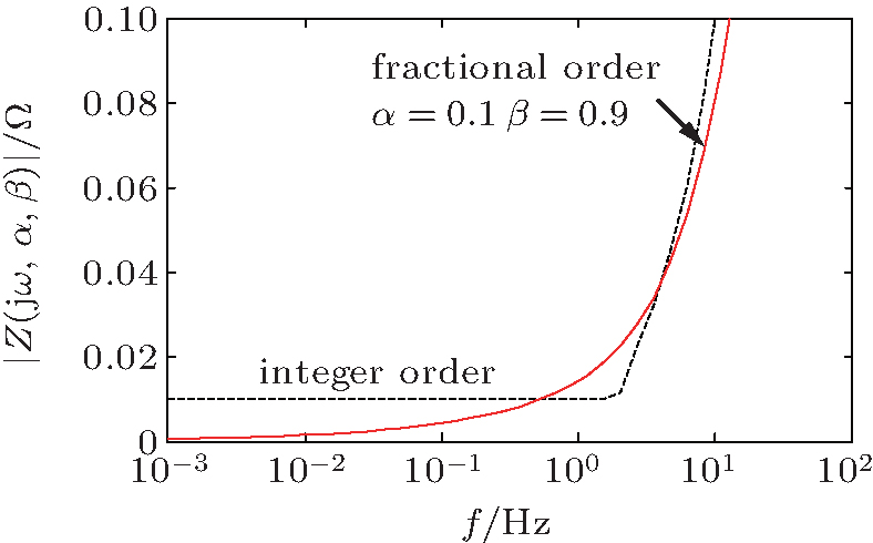 | Fig. 16. Absolute values of the impedance of the integer order and fractional-order filter circuit network with L = 0.01 and C = 100. |
The size and weight of the conventional filters are large with low operating frequency because of the necessary bulk capacitance and inductance, which is a major drawback of the conventional filters. Therefore, minimizing the capacitance and inductance as much as possible is of realistic significance to minimize the size and weight of the filters.
From Fig. 17, as for the fractional-order filter circuit network, the amplitude– frequency characteristic curve is much flatter in the passing band, and the selectivity of the octave is better in the transition region. Moreover, the numerical results show a better filtering characteristic of the fractional-order filter circuit network. Besides, the value of LC of the conventional filter circuit network is twice as great as that of the fractional-order filter circuit network. Therefore, the smaller capacitance and inductance are employed to satisfy requirements in practical applications, which can minimize the size and weight of the filters. In other words, it can remedy the defect of the conventional filters in the large size and weight.
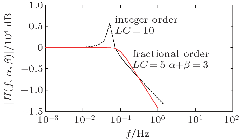 | Fig. 17. Amplitude– frequency characteristics of the integer order and fractional-order of the filter circuit network. |
In this work, we systematically studied the new laws and fundamentals of the fractional-order filter circuit network. From the point of view of the circuit, the effects of the system variables on the impedance characteristics and phase characteristics are systematically analyzed, which show many interesting phenomena. Specifically, the smaller inductance value power loss and zero phase can be obtained under special circumstances. In addition, the graphic model is presented to describe the effects of the two extra parameters on the impedance and phase characteristics. Furthermore, we studied the amplitude– frequency characteristics and phase– frequency characteristics in detail, and the better filtering properties are realized with the order less than 4, which are not possible for the conventional filter circuit network. Also, the effects of the number of filter units and fractional orders on the cut-off frequency are presented, and a critical cut-off frequency is obtained. Finally, two applicable examples are provided to show the better filter properties of the fractional-order filter circuit network.
In the future, we will continue to study the fractional-order high-pass filter circuit, band-pass filter circuit, and band rejection filter circuit networks in order to propel the industrial application of the fractional devices.
| 1 |
|
| 2 |
|
| 3 |
|
| 4 |
|
| 5 |
|
| 6 |
|
| 7 |
|
| 8 |
|
| 9 |
|
| 10 |
|
| 11 |
|
| 12 |
|
| 13 |
|
| 14 |
|
| 15 |
|
| 16 |
|
| 17 |
|
| 18 |
|
| 19 |
|
| 20 |
|
| 21 |
|
| 22 |
|
| 23 |
|
| 24 |
|
| 25 |
|
| 26 |
|
| 27 |
|
| 28 |
|