The solidification microstructure determines the properties of the final product. The directional solidification of binary alloys can produce planar, cellular, and dendritic interfaces.^{[1– 12]} The transition from planar to cellular interface can be well established by the Mullins– Sekerka instability theory.^[1] When the growth velocity V exceeds a threshold value V_c, the planar interface transients into a steady state cellular microstructure of wavelength λ _c. The depth of the cellular groove can be short, that is: shallow cell. A cellular groove can also be long, that is: deep cell. For even higher velocities, deep cells change into dendrites. The cell-to-dendrite transition (CDT) has been investigated for decades. However, the criterion of transition from a cellular to a dendritic microstructure has not been well established. Kurz and Fisher^[2] have proposed that V_cd = V_c/k₀ (V_cd = growth velocity of cellular– dendrite transition, V_c = planar growth stability limit, and k₀ = solute partition coefficient). Trivedi^[3] presented a minimum in the solute Peclet number p, which supported Kurz and Fisher (KF) criterion. Laxmanan et al.^[4] concluded that the KF criterion was doubtful, except for succinonitrile-acetone (SCN-ace) and Al– 2%   Cu alloys. Other alloys, such as SCN– Salol and Pb– Sn, did not support the KF criterion.

The onset of the sidewise instability has recently been investigated through the examination of the local spacing λ _cd of the CDT by Georgelin and Pocheau, ^[8] and Trivedi et al.^{[9, 10]} They found that cells and dendrites coexist over a range of velocities under fixed temperature gradient G and initial composition C₀. Within the transition zone, a critical spacing λ _cd is found, under which dendrites transform into cells and above which cells transform to dendrites. Georgelin and Pocheau^[8] analyzed an expression of the critical side-branching spacing, that is . Teng et al.^[10] presented a different expression: , where A is a constant, D_l is the diffusion coefficient, and Γ is the Gibbs– Thomson coefficient. They also concluded that the CDT initiates when the maximum cell spacing λ _{c, max} equals λ _cd. At the end of the CDT, the minimum dendrite spacing λ _{d, min} = λ _cd. According to λ _{c, max} = λ _cd, one can obtain the general expression for the lower limit of the CDT. Gurevich et al.^[23] have shown that there is a major difference between two- and three-dimensional configurations in the PF simulations. Furthermore, it was shown that the CDT is extremely sensitive to anisotropy.^{[23, 31]} Echebarria et al. ^[24] have found that the CDT cannot be understood by the phase field model without taking into account the thermodynamic noise.

To obtain a deep understanding of the CDT, the accuracy of the expressions of λ _{c, max}, λ _{d, min}, and λ _cd should be quantitatively examined to void incorrect formulas. The relationship among λ _cd, G, V, and C₀ has been quantitatively established by thin-film experiments. However, in experiments, the physical parameters, such as the Gibbs– Thomson coefficient Γ , the solute diffusivity D_l, the solute partition coefficient k₀, and the liquidus slope m_l, cannot be exhaustively surveyed. To quantitatively examine the influence of physical parameters on the CDT, numerical simulation is the only option. The phase-field model^{[13– 26]} has a nontrivial computational challenge to survey this problem. In this paper, a quantitative cellular automaton (CA) model^{[32– 35]} is used to investigate the influence of physical parameters on the CDT in directional solidification. In this paper, various CDT morphologies are simulated with different strengths of physical parameters while keeping the other parameters unchanged.

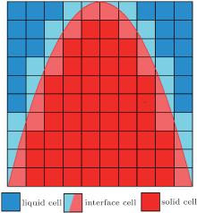
The computational domain is divided into a Cartesian grid. Each grid, which is also called a cell, is characterized by the following three states: liquid, solid, and interface, as seen in Fig.  1. To govern the transition of cell states, a capture rule is needed to control the evolution of different states. A solid fraction (i.e. solid cell f_s = 1, liquid cell f_s = 0, and interface cell 0 < f_s < 1) is introduced to implicitly capture the solid– liquid interface. The growth of solid fractions can be calculated according to the interface kinetics, which is also based on the algorithms of the interface curvature calculation and the thermal or mass transport calculation. The thermal and mass transport calculation methods can be found elsewhere.^{[28– 30]} The following subsections focus on the capture rule, interface curvature calculation, and the interface growth kinetics.

Fig.  1.

	Figure Option ViewDownloadNew Window
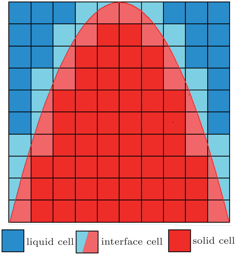	Fig.  1. The scheme of solid– liquid interface in CA model: liquid cell, interface cell, and solid cell.

The alloys for the simulations of the CDT are succinonitrile– 0.1  mol%   acetone (SCN– 0.1  mol%   ace) and SCN– 0.2  wt%   Salol, the thermal physical parameters are shown in Table  1.

Table 1.

Table 1.

Table 1. Thermal physical parameters of succinonitrile (SCN), SCN-acetone, and SCN-Salol. Parameters Values Succinonitrile latent heat (L) 3.705× 103  J· mol− 1 melting point (Tm) 331.233  K heat capacity (Cp) 160.15  J· mol− 1· K− 1 thermal diffusivity (α ) 1.134× 10− 7m2· s− 1 Gibbs– Thomson coefficient (Γ ) 6.62× 10− 8  m· K Succinonitrile-acetone diffusion coefficient in the liquid (Dl) 1.27× 10− 9  m2· s− 1 liquidus slope (ml) – 2.16  K· mol− 1· pct− 1 equilibrium partition coefficient (k0) 0.103 Succinonitrile-Salol diffusion coefficient in the liquid (Dl) 0.8× 10− 9  m2· s− 1 liquidus slope (ml) – 0.68  K· wt− 1· pct− 1 equilibrium partition coefficient (k0) 0.16

Table 1. Thermal physical parameters of succinonitrile (SCN), SCN-acetone, and SCN-Salol.

The computational domain is 256  μ m× 2048  μ m for the 2D model, and the mesh size is 1.0  μ m. If the simulation needs more resolution, then the computational domain of 512  μ m× 4096  μ m can be used. At the beginning of the simulations, the bottom of the computational domain is a planar interface.

According to the KF criterion, V_cd = V_c/k₀ = D_lG/(Δ T₀k₀) = D_lG/[m_lC₀(k₀ − 1)], and Γ has no effects on the CDT.

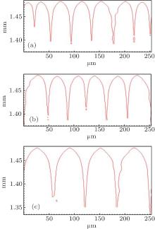
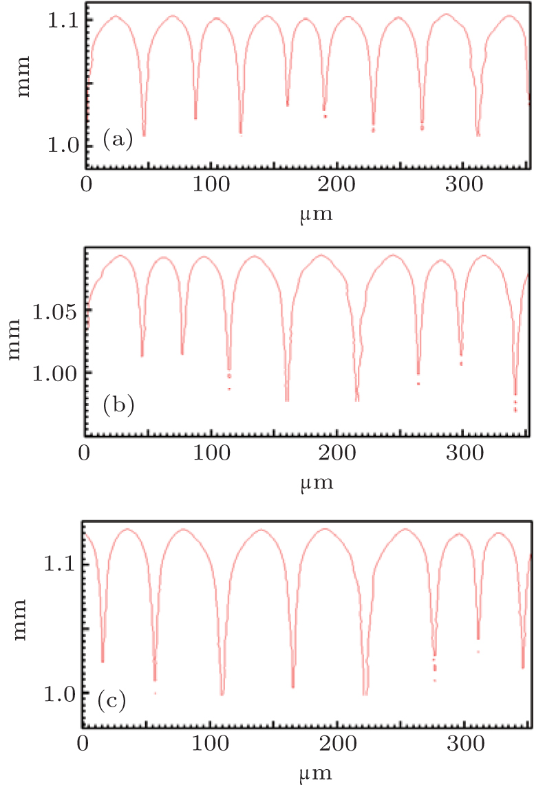
Figure  2 shows the simulation results with different Γ under unchanged conditions of V = 100  μ m/s, G = 15  K/mm, C₀ = 0.1  mol% , m_l = − 2.16  K/mol% , k₀ = 0.103, and ɛ = 0.005. When Γ increases from 3.2× 10^{− 8}  m· K to 9.6× 10^{− 8}  m· K, both the cell and the dendrite spacings increase. However, it can be obviously seen that the changing of Γ has no effects on the CDT. The influence of Γ on the CDT agrees well with the KF criterion.

Fig.  2.

	Figure Option ViewDownloadNew Window
	Fig.  2. The simulated morphologies of SCN-ace alloy with different strengths of Gibbs– Thomson coefficient Γ . (a) Γ = 3.2 × 10− 8  m· K, G = 15  K/mm, V = 100  μ m/s, (b) Γ = 6.4 × 10− 8  m· K, G = 15  K/mm, V = 100  μ m/s, (c) Γ = 9.6 × 10− 8  m· K, G = 15  K/mm, V = 100  μ m/s.

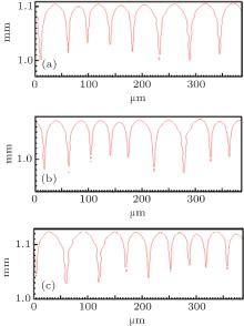
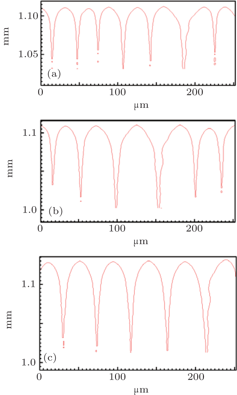
By using the same strategy, the solute diffusivity D_l, the initial composition C₀, and the liquidus slope m_l are also examined by the CA simulations, as shown in Figs.  3– 5. The corresponding changes in pulling velocities V or temperature gradient G are calculated according to the KF criterion. The simulation results show that the three physical parameters: m_l, C₀, and D_l also agree well with the prediction of the KF criterion.

Fig.  3.

	Figure Option ViewDownloadNew Window
	Fig.  3. The simulated morphologies of SCN-ace alloy with different strengths of the solute diffusivity Dl, while keeping Dl/V constant. (a) Dl = 0.635 × 10− 9  m2/s, G = 15  K/mm, V = 50  μ m/s, (b) Dl = 1.27 × 10− 9  m2/s, G = 15  K/mm, V = 100  μ m/s, (c) Dl = 1.91 × 10− 9  m2/s, G = 15  K/mm, V = 150  μ m/s.

Fig.  4.

	Figure Option ViewDownloadNew Window
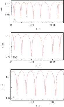
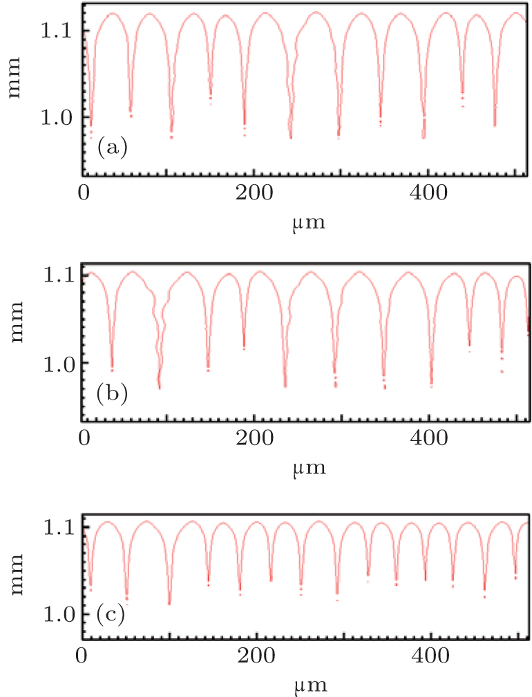
	Fig.  4. The simulated morphologies of SCN-ace alloy with different strengths of the initial composition C0, while keeping G/C0 constant. (a) C0 = 0.20, G = 30  K/mm, V = 100  μ m/s, (b) C0 = 0.1, G = 15  K/mm, V = 100  μ m/s, (c) C0 = 0.0667, G = 10  K/mm, V = 100  μ m/s.

Fig.  5.

	Figure Option ViewDownloadNew Window
	Fig.  5. The simulated morphologies of SCN-ace alloy with different strengths of the liquidus slope ml, while keeping mlV constant. (a) ml = − 1.44, G = 15  K/mm, V = 150  μ m/s, (b) ml = − 2.16, G = 15  K/mm, V = 100  μ m/s, (c) ml = − 2.88, G = 15  K/mm, V = 75  μ m/s.

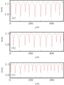
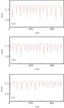
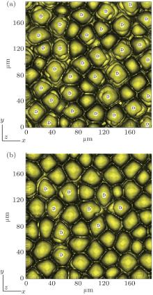
However, the solute partition coefficient k₀ is very exceptional, which is the main finding of this paper. During the simulations, k₀ was continually  increased from 0.04 to 0.16 by an interval of 0.01. The pulling velocities were set close to the prediction of the KF criterion. Figures  6 (SCN-0.1  mol%   ace) and  7 (SCN-0.2  wt%   Salol) show the influence of k₀ on the CDT, in which only k₀ = 0.04, 0.10, and 0.16 are presented. The simulation results show that when k₀ is small, the simulated morphologies are the CDT; and, when k₀ is large, the morphologies are cellular. Figure  8 is the 3D simulation of the SCN-0.1  mol%   ace with different k₀. By comparing the 2D and 3D simulation results, it can be concluded that a similar influence pattern of k₀ on the CDT is obtained. Overall, both the 2D and the 3D CA simulations show that the KF criterion is only validated when k₀ is small.

Fig.  6.

	Figure Option ViewDownloadNew Window
	Fig.  6. The simulated morphologies of SCN-ace alloy with different strengths of the solute partition coefficient k0, while keeping (1 − k0)V constant. (a) k0 = 0.04, G = 15  K/mm, V = 93.87  μ m/s, (b) k0 = 0.10, G = 15  K/mm, V = 100.00  μ m/s, (c) k0 = 0.16, G = 15  K/mm, V = 106.99  μ m/s.

Fig.  7.

	Figure Option ViewDownloadNew Window
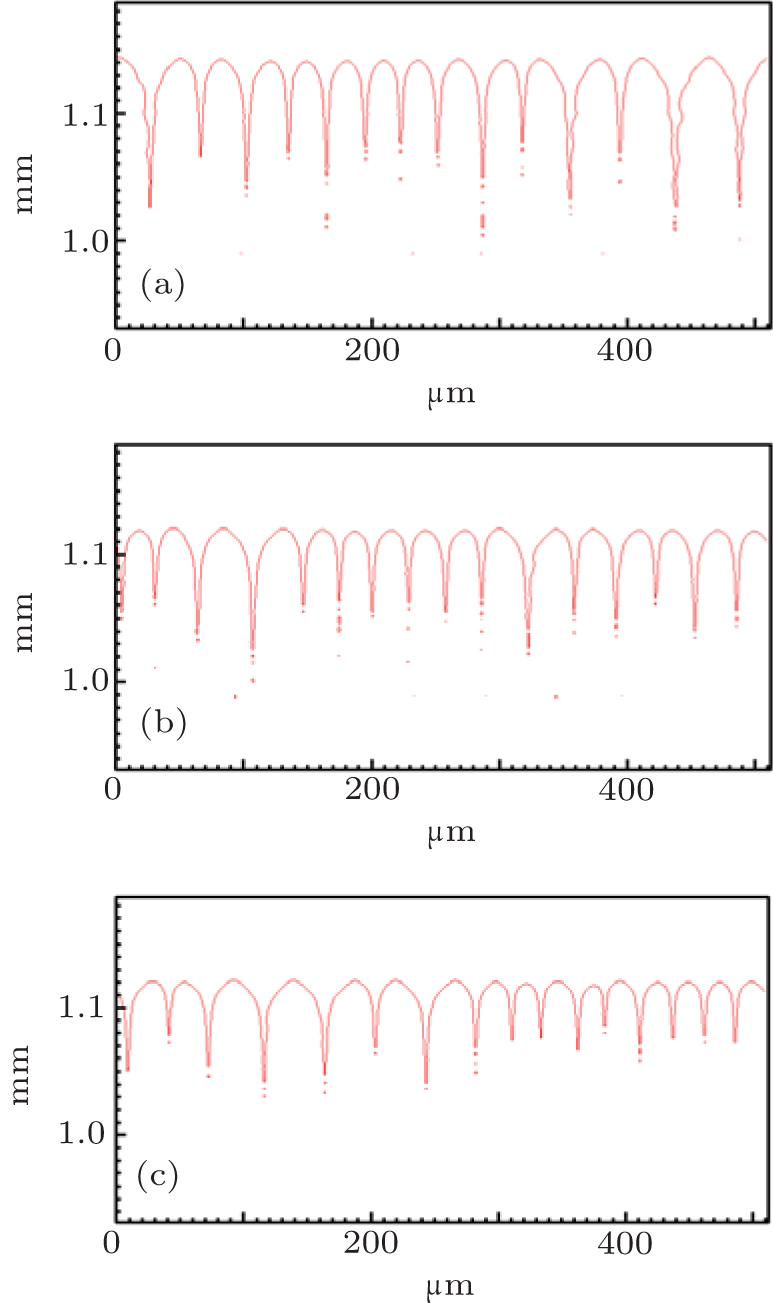	Fig.  7. The simulated morphologies of SCN-Salol alloy with different strengths of the solute partition coefficient k0, while keeping (1 − k0)V constant. (a) k0 = 0.04, G = 15  K/mm, V = 93.91  μ m/s, (b) k0 = 0.10, G = 15  K/mm, V = 100.00  μ m/s, (c) k0 = 0.16, G = 15  K/mm, V = 107.04  μ m/s.

Fig.  8.

	Figure Option ViewDownloadNew Window
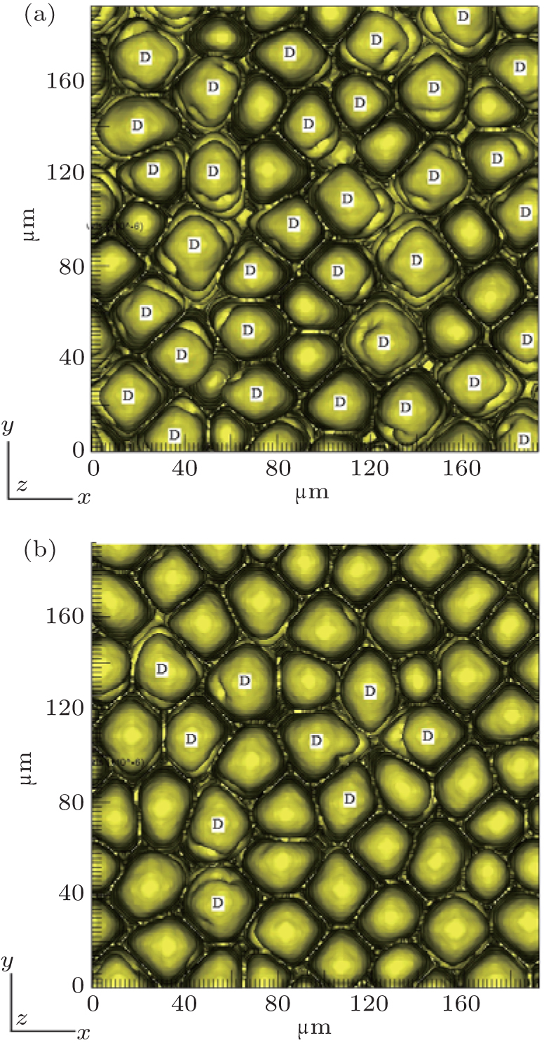	Fig.  8. The 3D simulations of the CDT for SCN-ace alloy with solute partition coefficient conditions: (a) k0 = 0.10, G = 15  K/mm, V = 100  μ m/s, (b) k0 = 0.20, G = 15  K/mm, V = 112.5  μ m/s.

To quantitatively understand the CDT, the relationship between λ _{c, max} and λ _cd should be analyzed. Teng et al.^[10] have presented an expression of the λ _cd by investigating through a thin film experiment

and Georgelin and Pocheau have presented a different expression of the λ _cd

Hunt and Lu^[27] presented a rough expression for the cell spacings. The phase field simulations^{[13, 23]} evidenced that the relationship between the maximum finger spacing and the pulling velocity is . Based on the phase field simulations, the Hunt– Lu expression is modified into

where B₁ is constant.

Based on the investigations in present CA simulations and the KF criterion, the critical velocity V_cd of the CDT should follow the expression

where B₂ is constant, f (ɛ ) and g (k₀) are the unknown expressions of ɛ and k₀.

By solving λ _cd = λ _{c, max}, one can obtain the expression of V_cd. Since equations  (6) and (7) have the same V^{− 1/2}, the V_cd cannot be obtained based on the two formulas. Equation  (5) is selected to be a more appropriate formula to describe the λ _cd. To get consistent results with Eq.  (8), equations  (5) and  (7) are modified slightly as

where B₃ and B₄ are constant.

The modifications are based on the following considerations. The in Eq.  (5) is modified into in this paper to obtain a consistent result. In Trivedi’ s experiment, ^[10] it is found that , which is also close to , since it is difficult to accurately measure C₀ in the experiments. Using the data in Fig.  2, the relationship between λ _cd and Γ is established to λ _cd ∝ Γ ^1/3, as shown in Fig.  9. The relationship of λ _{c, max} ∝ Γ ^1/3 can also be obtained in Fig.  9. Hence, the expression of Γ should be modified into Γ ^1/3, as seen in Eq.  (7). In Eq.  (7), the temperature gradient G^{− 1/6} is a guess that is made to have a consistent formula.

Fig.  9.

	Figure Option ViewDownloadNew Window
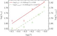
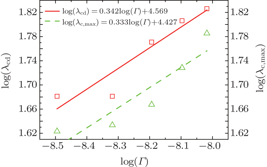	Fig.  9. Plots of log(λ cd)– log(Γ ) and log(λ c, max)– log(Γ ) based on the data in the present CA simulations.

Overall, based on Eqs.  (8)– (10), one can get a self-consistent relationship among λ _{c, max}, λ _cd, and V_cd. By solving λ _cd = λ _{c, max}, we can obtain the exact expression of V_cd. However, the influence of the interface energy anisotropy ɛ on the λ _{c, max} and λ _cd are still unknown. Therefore, the influences of k₀ and ɛ should be quantitatively investigated later.

In conclusion, the influences of the physical parameters (Γ , D_l, m_l, C₀) on the cell-to-dendrite transition in directional solidification are investigated by using CA simulations. It is evidenced that Gibbs– Thomson coefficient Γ has no effects on the CDT. It is also found that the influences of the physical parameters (D_l, m_l, C₀) exactly follow the Kurz and Fisher (KF) criterion. The most important finding in this paper is that when k₀ is small, the influences of k₀ on the CDT agree with the KF criterion; and, when k₀ is larger than 0.16, the V_cd is higher than the prediction of the KF criterion. The special performance of k₀ on the CDT could explain why SCN-ace and SCN-Salol have different behaviors on the CDT. Based on the simulation results, the expressions of the cell spacing λ _{c, max} and the critical spacing λ _cd are modified to give a consistent formula to predict the CDT.