

Load-redistribution strategy based on time-varying load against cascading failure of complex network
[Liu Juna) , Xiong Qing-Yu†b), c)  , Shi Xin
a) , Wang Kaia) , Shi Wei-Rena) ]
, Shi Xin|
|


†Corresponding author. E-mail: cquxqy@163.com
*Project supported by the National Basic Research Program of China (Grant No. 2013CB328903), the Special Fund of 2011 Internet of Things Development of Ministry of Industry and Information Technology, China (Grant No. 2011BAJ03B13-2), the National Natural Science Foundation of China (Grant No. 61473050), and the Key Science and Technology Program of Chongqing, China (Grant No. cstc2012gg-yyjs40008).
Cascading failure can cause great damage to complex networks, so it is of great significance to improve the network robustness against cascading failure. Many previous existing works on load-redistribution strategies require global information, which is not suitable for large scale networks, and some strategies based on local information assume that the load of a node is always its initial load before the network is attacked, and the load of the failure node is redistributed to its neighbors according to their initial load or initial residual capacity. This paper proposes a new load-redistribution strategy based on local information considering an ever-changing load. It redistributes the loads of the failure node to its nearest neighbors according to their current residual capacity, which makes full use of the residual capacity of the network. Experiments are conducted on two typical networks and two real networks, and the experimental results show that the new load-redistribution strategy can reduce the size of cascading failure efficiently.
Complex networks are all around us, they are not strange to us, for example, traffic networks, [1, 2] power grids, [3– 6] the Internet, [7, 8] computer networks, [9] and so on; they can all be described by complex networks. With rapid economic and social development, some problems are getting more and more serious in these infrastructure networks, such as traffic congestion, blackout, and so on. Du et al.[10] introduced a shortest-remaining-path-first queuing strategy into a network traffic model, which is helpful for designing optimal networked-traffic systems. Liu et al.[11] proposed a routing strategy based on the gravitational field of the node and the routing awareness depth, which can reduce traffic jams and improve the ability of the network to resist congestion. Considering the scale-free property in real networks, Liu et al.[12] adopted the scale-free network to represent the individual interactions in the particle swarm optimization (PSO) algorithm and explored the dynamical searching process microscopically, finding that the cooperation of hub nodes and non-hub nodes play a crucial role in optimizing the convergence process. It has the implication in controlling a variety of dynamical processes taking place on complex networks. The robustness of networks is one of the central issues in complex network research. Cascading failure can cause great damage to complex networks, which can be described as follows. The loads of the network are time-varying, and the capacities of the network are limited. The failure of one node can cause the redistribution of loads, and this redistribution may make the loads of some nodes exceed their capacities, which leads to further failures and load-redistribution and finally to a cascading breakdown of the whole network. There has been a lot of research related to cascading failure. This issue is crucial for infrastructure networks, which our modern human society greatly relies on. Duan et al.[13] proposed a novel node importance indicator based on the information about cascading failures and analyzed the node importance evolution mechanism in-depth, which is helpful to improve the network robustness.
There are also many models proposed to improve network robustness against cascading failure. Motter et al.[14] assumed that the load is exchanged between every pair of nodes and transmitted along the shortest path connecting them. The load of a node is defined as the betweenness of the node. The removal of nodes in general changes the distribution of the shortest paths. They assume that the capacity of a node is proportional to its initial load, which is adopted in many researches.[15– 19] The definition of the load and the load-redistribution strategy require each node to master the whole information of the network though the global load-redistribution strategy can obtain good results. Therefore, it tends to be used in small complex networks. For large scale networks, the global information is hard to obtain. Moreover, the load may not be transmitted along the shortest path. Then, Wang et al.[20] proposed a cascading failure model based on the local preferential redistribution rule of the load of the failure node, defining the initial load of a node as the function of the degree of the node. Wang et al.[15] put forward a local weighted flow redistribution rule to investigate the cascading failure on weighted complex networks. They assumed that the additional flow received by an edge is proportional to its weight (flow). Ren et al.[21] presented a model of cascading failure, and it adopts a new redistribution strategy based on the difference between capacity and the initial load. Duan et al.[22] proposed a new cascading model based on a tunable load redistribution model. It can achieve better robustness against cascading failure than the previous model by adjusting the redistribution range and heterogeneity. Chen et al.[23] studied the influences of network coupling strength, subnetwork edge, and coupling edge of interdependent networks on the network robustness. These strategies based on the local information rather than global information are more suitable for large scale networks, but in these strategies the load of the failure node (or edge) is redistributed to its neighbors according to their initial load or initial residual capacity rather than their current load or their current residual capacity. It will lead to an unreasonable redistribution of loads, which will easily lead to further failures and eventually spread over the entire network. In fact, the loads of the real network are constantly changing, such as the traffic in a traffic network, the power consumption in a power grid, and so on. Then, the residual capacity of the node will change along with the time-varying load of the node, so it is necessary to propose a load-redistribution strategy based on local information considering the time-varying loads of a network.
In view of the above problems, we propose a new load-redistribution strategy, which is able to make full use of the residual capacity of the network. The experimental results show that it can well improve the network robustness against cascading failure, especially when the loads of the network are constantly changing.
A new model considering a time-varying load is proposed based on the load-capacity model. There are three main elements, including the initial load of the node, the capacity of the node, and the load-redistribution strategy.
In many researches, the initial load of the node is defined as the total number of shortest paths passing through this node. The definition can well describe the initial load of the node, but it needs the global information, and the global information is not readily available in a large-scale network. Wang et al.[24] defined the initial load of the node as the product of the degree of the node and the sum of the degree of its neighbors, which is in positive correlation with betweenness centrality.[25] Therefore, this definition can describe the initial load of the node as well as betweenness centrality. Moreover, it is based on the local information instead of the global information, so the initial load 
where ki is the degree of node i, Γ i is the set of neighbors of node i, α is a tunable parameter and governs the strength of the initial load, and N is the number of nodes in a complex network.
The capacity of a node is the maximum load that the node can deal with. As is well known, the larger the node capacity is, the stronger the network robustness is. However, the capacity of a node is severely limited by the cost in real networks. Thus, Motter and Lai[14] assume that the capacity Ci of node i is proportional to its initial load

where β > 0 is the tolerance parameter, and N is the number of nodes in a complex network. This definition is commonly used in many researches. In this paper, we also use this definition.
The strategies based on the local information mentioned in Section 1 are all based on the fixed factors, including the initial load, capacity, and initial residual capacity. Moreover, these strategies assume that the load of a node is always its initial load no matter when the node is destroyed. The strategy based on the initial residual capacity can be described as

The strategy based on the initial load is defined as

In this paper, we assume that the capacity Ci of node i is proportional to its initial load


from which one can see that Eqs. (3) and (4) are equivalent and we call these two strategies fixed strategy (FS).
However, in real networks, the load of a node is constantly changing rather than remaining the same due to the existence of the disturbance variable. For example, in a traffic network, the traffic varies with the time of the day. Generally speaking, there is more traffic both in the morning and at dusk. If at this time one node of the traffic network fails, it will induce further failures more easily than at ordinary times and eventually lead to a cascading breakdown of the entire network. Similarly, in a power grid, the power consumption varies along with the time. Therefore, a strategy based on local information considering a time-varying load is needed to improve the robustness of the large scale networks.
In this paper, we propose a load-redistribution strategy considering the time-varying load and the time-varying residual capacity against cascading failure. Here, we call this strategy the time-varying strategy (TVS). The time-varying load Li(0) of node i is defined as

where Δ l is the disturbance variable, it can be defined according to the variation trend of the load. Here, in order to explore the robustness of the model, for simplicity, 
The load of failure node i is redistributed to the nearest neighbors of node i in proportion of the current remaining capacity, as
where Cj is the capacity of node j, Lj(t) is the load of node j at the time step t, q is the number of time steps before the cascading process stops, j is the nearest neighbor of node i, and Γ i is the set of nearest neighbors of node i.
According to this principle, the extra load Δ Lji that node j should obtain from the failure node i is

so at the time step t + 1, if Lj(t) ≤ Cj, the load of node j is

where Γ j is the set of nearest neighbors of node j. If Lj(t + 1) > Cj, node j is removed from the network, and the load Lj(t + 1) of node j is redistributed to its nearest neighbors, and this load-redistribution may lead to new overload failure. This cascading process may stop after a few steps, while it could also spread over the entire network.
To discuss the cascading failure more easily, we introduce Pi to evaluate the proportion of failure nodes due to the removal of node i

where Fi is the number of failure nodes caused by the removal of node I, N is the total number of nodes in the complex network. Obviously, 0 ≤ Fi ≤ N − 1.
Then, the average proportion of failure nodes due to the removal of one node of the entire network can be described as

The lower the proportion of failure nodes is, the more robust the whole network is against cascading failure.
The topology of the network plays an important role in studying the cascading failure of the network.[15, 20] Networks with different topology may show different anti-destroying abilities. In this paper, we consider two typical complex networks, including BA networks[26] and WS networks.[27] It has been found that the small-world and scale-free properties are ubiquitous in nature and human society.[28]
BA network proposed by Barabá si and Albert[26] is a scale-free network, and many real networks display a scale-free feature, so it is significant to discuss the cascading failures under scale-free networks. However, some networks are homogeneous. In order to structure these networks, we consider WS networks with a small-world property. The two typical complex networks used in this paper were both generated by Pajek. For each network, the number of nodes N = 1000 and ⟨ k⟩ = 8.
Although typical model networks are useful in understanding how real networks behave, they cannot catch many of the structural properties of real systems. Therefore, we also consider some real-life complex networks including the US power grid network (UPG)[29] and the USA airport network (UAN).[30] The UPG is the high-voltage power grid in the Western States of the United States of America. There are 4941 nodes and 6594 edges in the power grid of the western United States. The nodes are transformers, substations, and generators, and the ties are high-voltage transmission lines. The UAN is the network of the 500 busiest commercial airports in the United States. A tie exists between two airports if a flight was scheduled between them in 2002.
In this research, to compare our load-redistribution strategy (TVS) with FS on four networks, we remove only one node i initially and calculate the proportion of failure nodes Pi after the cascading failure process is over. The P is calculated according to Eq. (11) and each experimental result is the average value of 10 realizations. The experiment is divided into two parts. One is under the condition that ε i = 0, the other is under the condition that ε i is a random number between − 1 and 1.
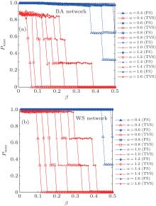
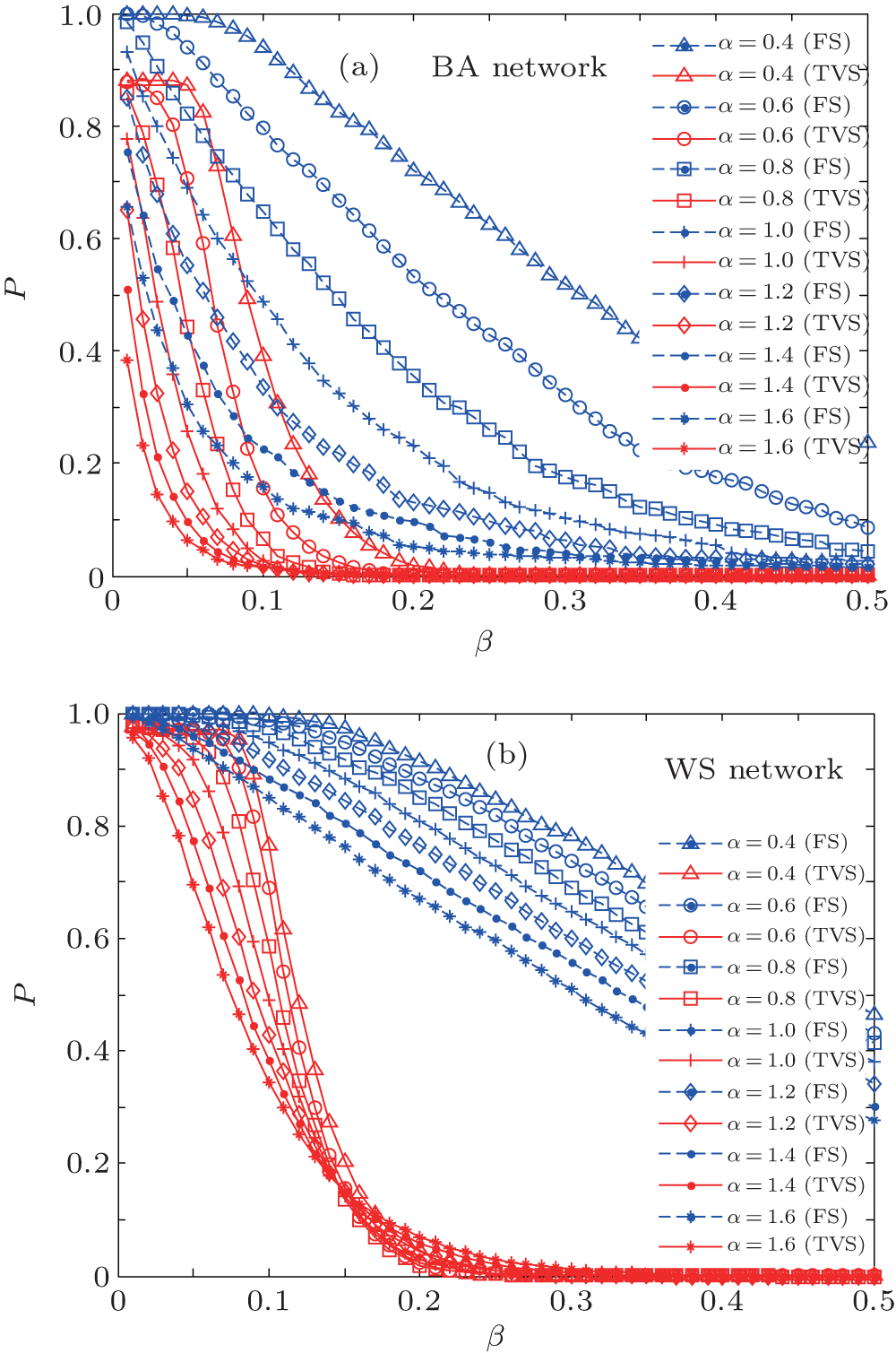
Firstly, we assume that the loads of the nodes in complex networks are always their initial loads (ε i = 0). In this condition, we compare TVS with FS under a BA network and a WS network. Figure 1 shows the relationship between β and P under different strategies. From Fig. 1(a), one can see that in the BA network the average proportion of failure nodes due to the removal of one node is becoming lower with the increase in β . There will be no cascading failure when β ≥ β T, where β T is the critical threshold at which a phrase transition occurs from normal state to collapse. It can also be seen that the proportion of failure nodes based on TVS is lower than that based on FS for the same α when β is a constant value and β < β T. Furthermore, one can also see that in the BA network the average proportion of failure nodes P is becoming lower with the increase of α . Figure 1(b) shows the relationship between β and P under different strategies in the WS network. From Fig. 1(b), one can also see that the proportion of failure nodes based on TVS is lower than that based on FS. In addition, one can see that the results with bigger α are better than those with smaller α in the beginning, while with the increase of β the results with smaller α tend to be better than those with bigger α . It is not accidental. According to Eq. (1), the smaller the value of α is, the more homogeneous the load of the nodes is. There exists a small enough interval of β when α = 0.4, in which the network can change from normal to cascading failure of the entire network immediately. While with the increase of α , the homogeneousness of the load is becoming more and more insignificant and there are no such small intervals of β when α = 1.6, which lead to a slow decrease of P though at the beginning P with α = 1.6 is smaller than P with α = 0.4, so it is reasonable that the results of α = 0.4 are better than the results of α = 1.6 when β > 0.13.
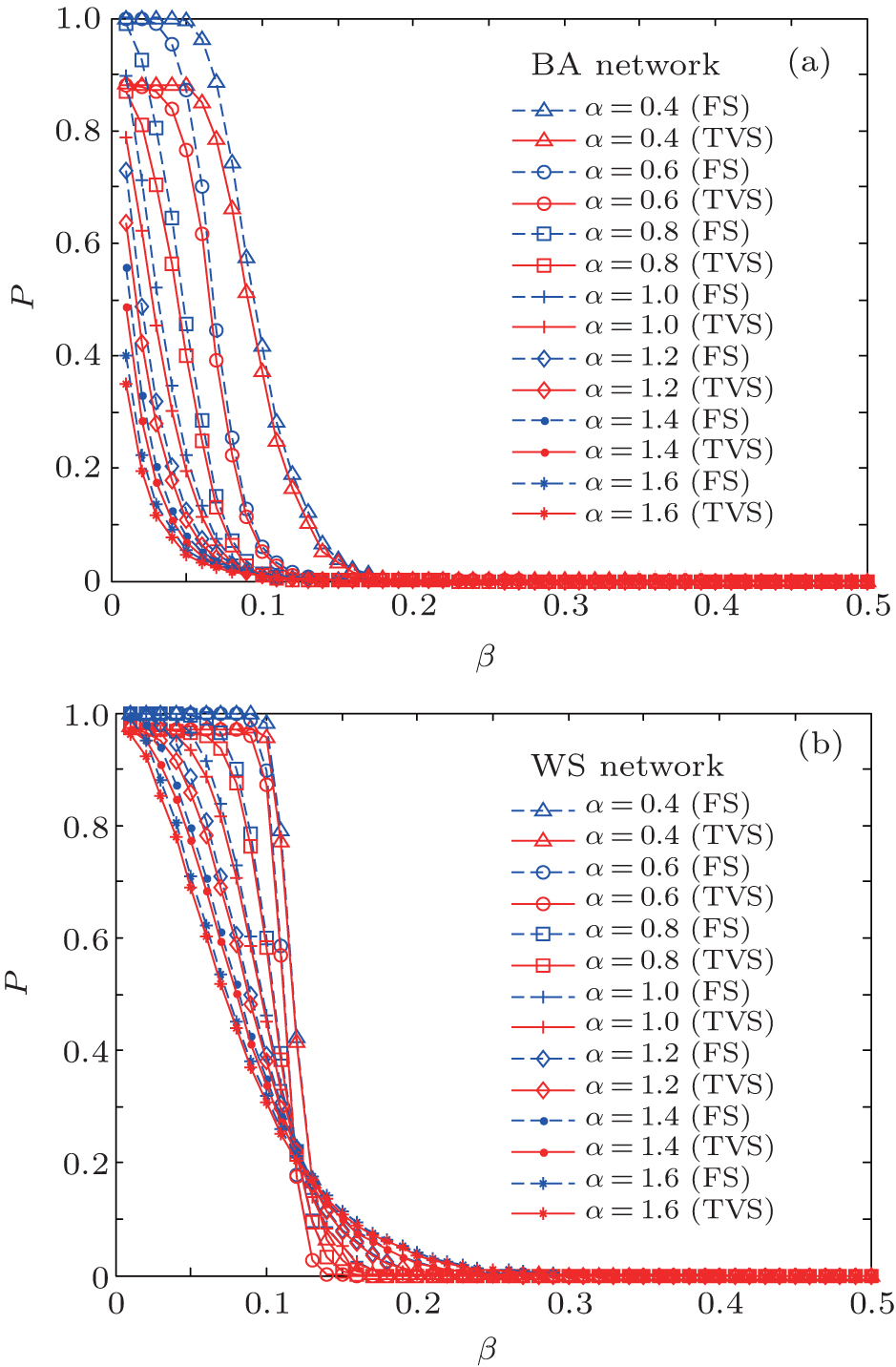 | Fig. 1. The relationship between β and P under different strategies in two typical networks (ε i = 0): (a) BA network, (b) WS network. |
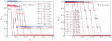
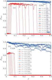
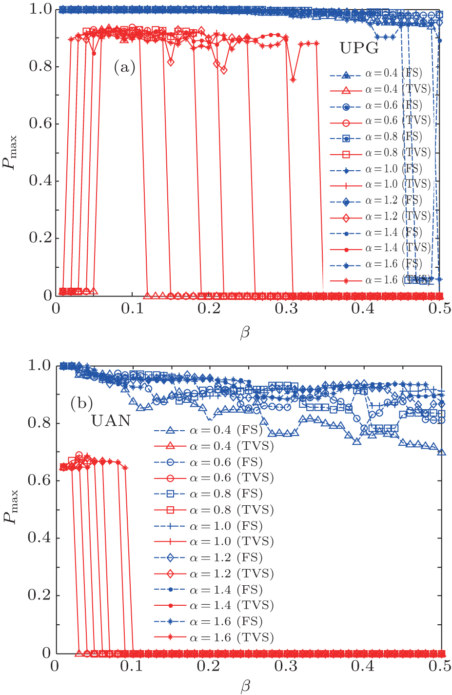
To further illustrate the effectiveness of TVS, we remove the node with the highest load of four networks (two typical networks and two real networks) and calculate the proportion of failure nodes Pmax. The results are shown in Figs. 2 and 3. From Fig. 2, one can see that TVS also performs competitively well. Moreover, in Fig. 2, one can see that Pmax is becoming higher with the increase of α . Compare Fig. 2 with Fig. 1, one can see that Pmax is the highest when α = 1.6 and Pmax is the lowest when α = 0.4 in Fig. 2, while in Fig. 1, P is the highest when α = 0.4 and P is the lowest when α = 1.6. It is known that the load heterogeneity of the network is increasing with the increase of α . It has been commonly recognized that heterogeneous networks are extremely vulnerable to the failure of a high-load node. This explains the phenomenon in Fig. 2. However, P in Fig. 1 is the average proportion of failure nodes due to the removal of an arbitrary node of the entire network. when α = 1.6, the network has load heterogeneity and most of the nodes are low-load, the removal of these nodes hardly induces cascading failure, so the average value of the whole network is relatively small. While when α = 0.4, the loads of the network are homogeneous, the failure of any one node can induce cascading failure, so the average value of the whole network is relatively large. It explains the experimental result in Fig. 1. In Fig. 3, it shows the experimental results in two real networks (UPG and UAN). In UPG, one can see that the proportion of the failure node is not simply descending with the increase of β under the new load-redistribution strategy (TVS) when α = 0.4. On the contrary, Pmax ≈ 0.014 when β ≤ 0.05 and Pmax ≈ 0.9 when 0.06 ≤ β ≤ 0.11, which indicates that the lower capacity can make the network more robust against cascading failure sometimes under TVS. Similarly, there is the same phenomenon with other values of α . On the whole, TVS performs better than FS in UPG. In UAN, compared with FS, TVS also performs better in the same condition.
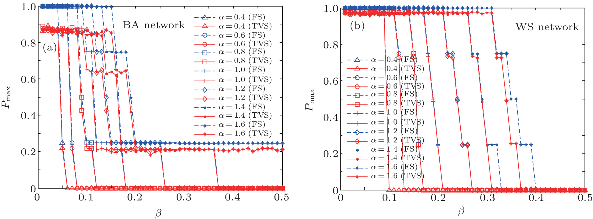 | Fig. 2. The relationship between β and Pmax under different strategies in two typical networks (ε i = 0): (a) BA network, (b) WS network. |
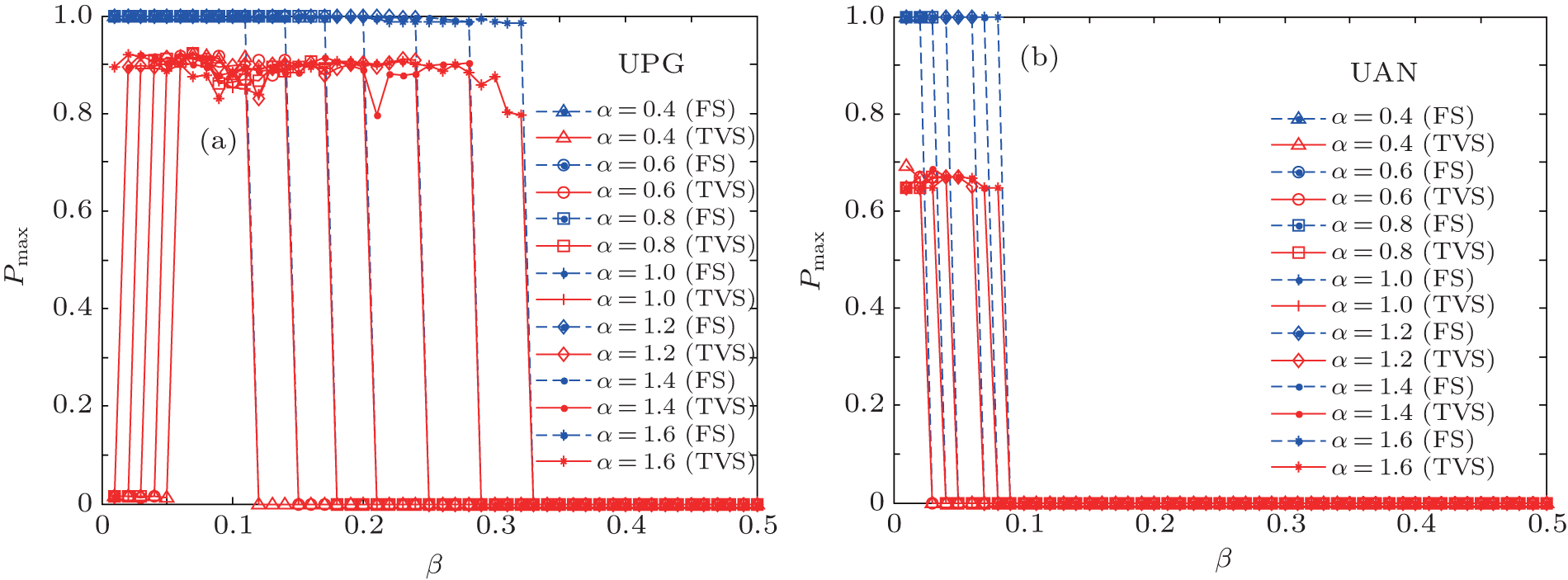 | Fig. 3. The relationship between β and Pmax under different strategies in two real networks (ε i = 0): (a) UPG, (b) UAN. |
Then, we assume that ε i is a random number between − 1 and 1 (− 1 ≤ ε i ≤ 1). A group of random sequences between − 1 and 1 is generated by MATLAB as

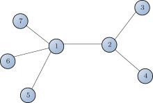
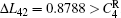
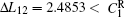
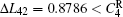
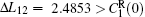
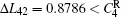
where N is the total number of nodes in the complex network. From Fig. 4, one can see that the cascading failure model based on FS cannot restrain the cascading failure efficiently and a lot of nodes lose their efficacy when the loads of nodes are ever-changing. On the contrary, the model based on TVS is able to reduce the avalanche size effectively in the same conditions. It indicates that some nodes’ failure can be avoided as long as the load of the failure node is redistributed reasonably. FS cannot make full use of the residual capacity of the network, while TVS is able to redistribute the loads of failure nodes based on the current residual capacity of intact nodes. It can be illustrated as follows. Figure 5 is a simple network. According to Eq. (1), we set α = 0.5, then 


 | Fig. 4. The relationship between β and P under different strategies in two typical networks (− 1 ≤ ε i ≤ 1): (a) BA network, (b) WS network. |
 | Fig. 5. A simple network. |
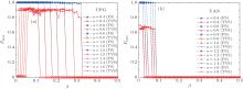
Similarly, to further illuminate the effectiveness of TVS, we remove the node with the highest load of two typical networks and two real networks and calculate the proportion of failure nodes Pmax. Figure 6 shows the relationship between β and Pmax under different strategies in two typical networks (BA network and WS network). As shown in Fig. 6(a), the model based on FS hardly restrains the cascading failure and almost all nodes in the BA network failed, while the model based on TVS is able to reduce the size of the cascading failure effectively in the same conditions. From Fig. 6(b), one can see that the model based on FS hardly restrains the cascading failure and almost all nodes in the WS network failed, while the model based on TVS is able to reduce the size of the cascading failure effectively in the same conditions. Figure 7 shows the experimental results of two real networks. In UPG, under FS, cascading failure spreads over the entire network and almost all nodes failed. However, the network can be more robust under TVS. In UAN, TVS also performs well. In a word, TVS performs better than FS in the condition that the load of a node is time-varying.
 | Fig. 6. The relationship between β and Pmax under different strategies in two typical networks (− 1 ≤ ε i ≤ 1): (a) BA network, (b) WS network. |
 | Fig. 7. The relationship between β and Pmax under different strategies in two real networks (− 1 ≤ ε i ≤ 1): (a) UPG, (b) UAN. |
In this paper, we propose a load-redistribution strategy (TVS) based on ever-changing load. Compared with those strategies based on global information, the current strategy only needs local information. It is more suitable for large scale networks. Different from FS, TVS is able to make full use of the residual capacity by considering the real-time loads of nodes rather than their initial loads. In real networks, the loads of nodes are not definite values. The assumption that the loads of nodes are always their initial loads is unreasonable, so TVS is more suitable for real networks compared with FS. The results of experiments on two typical networks (BA network and WS network) and two real networks (UPG and UAN) show that TVS performs better than FS in the same conditions, especially when − 1 ≤ ε i ≤ 1. The simulation results indicate that TVS can more reasonably redistribute the loads of failure nodes to their neighbors and more effectively reduce the avalanche size than FS.
| 1 |
|
| 2 |
|
| 3 |
|
| 4 |
|
| 5 |
|
| 6 |
|
| 7 |
|
| 8 |
|
| 9 |
|
| 10 |
|
| 11 |
|
| 12 |
|
| 13 |
|
| 14 |
|
| 15 |
|
| 16 |
|
| 17 |
|
| 18 |
|
| 19 |
|
| 20 |
|
| 21 |
|
| 22 |
|
| 23 |
|
| 24 |
|
| 25 |
|
| 26 |
|
| 27 |
|
| 28 |
|
| 29 |
|
| 30 |
|