


A new mixed subgrid-scale model for large eddy simulation of turbulent drag-reducing flows of viscoelastic fluids*
[Li Feng-Chen† , Wang Lu, Cai Wei-Hua]
, Wang Lu, Cai Wei-Hua]
|
|


†Corresponding author. E-mail: lifch@hit.edu.cn
*Project supported by the China Postdoctoral Science Foundation (Grant No. 2011M500652), the National Natural Science Foundation of China (Grant Nos. 51276046 and 51206033), and the Specialized Research Fund for the Doctoral Program of Higher Education of China (Grant No. 20112302110020).
A mixed subgrid-scale (SGS) model based on coherent structures and temporal approximate deconvolution (MCT) is proposed for turbulent drag-reducing flows of viscoelastic fluids. The main idea of the MCT SGS model is to perform spatial filtering for the momentum equation and temporal filtering for the conformation tensor transport equation of turbulent flow of viscoelastic fluid, respectively. The MCT model is suitable for large eddy simulation (LES) of turbulent drag-reducing flows of viscoelastic fluids in engineering applications since the model parameters can be easily obtained. The LES of forced homogeneous isotropic turbulence (FHIT) with polymer additives and turbulent channel flow with surfactant additives based on MCT SGS model shows excellent agreements with direct numerical simulation (DNS) results. Compared with the LES results using the temporal approximate deconvolution model (TADM) for FHIT with polymer additives, this mixed SGS model MCT behaves better, regarding the enhancement of calculating parameters such as the Reynolds number. For scientific and engineering research, turbulent flows at high Reynolds numbers are expected, so the MCT model can be a more suitable model for the LES of turbulent drag-reducing flows of viscoelastic fluid with polymer or surfactant additives.
In 1948, turbulent drag-reduction (DR) by polymer additives, the so-called Toms’ effect, [1] was first reported. It is well known that the addition of flexible long-chain polymers (or some kinds of surfactants discovered later on) into a turbulent flow of water or organic solvents at only a minute concentration can induce significant DR. In wall-bound turbulent flows of viscoelastic fluid, significant frictional DR has been repeatedly discovered.[2– 7] And in some cases, the DR can exceed 80%.[8] Many academic communities have paid much attention to this phenomenon after it was discovered, since this technique can straightforwardly save energy. The most suitable application for turbulent DR technique in daily life is a district heating/cooling circulation (DHC) system: an overall benefit including reduction of pumping power, decrease of pipe diameter, etc., can be obtained by addition of drag-reducing surfactant additives into a DHC system. However, apart from the fact that there is more to be known regarding turbulent drag-reducing flow by additives, such as the mechanisms of DR, turbulence scaling characteristics of drag-reducing flow, interactions between turbulence and microstructures in the solution, etc., there are already reliable and robust theoretical or numerical estimation tools for turbulent drag-reducing flows at Reynolds numbers as high as those required for application in real systems. This is one of the critical issues for drag-reducing additives to be utilized in industrial applications.
With the rapid development of computer hardware and software techniques, numerical simulations of turbulent drag-reducing flows have been carried out in many studies. Direct numerical simulation (DNS) is always the preferred approach for turbulent flows, including drag-reducing flows, since DNS can directly resolve all scales of turbulence in a turbulent flow without any models. Sureshkumar et al.[9] first used DNS to simulate a turbulent drag-reducing flow with the finitely extensible nonlinear elastic in the Peterlin approximation (FENE-P) model by using a pseudospectral method. Dimitropoulus et al.[10] then applied the pseudospectral method to simulate turbulent flows with polymer additives at various flow conditions. They found that for a Giesekus fluid the pseudospectral method is more suitable for high concentration solutions. After those pioneering efforts, more and more DNS studies have been carried out to investigate the detailed characteristics of drag-reducing flows and research the mechanism of the DR phenomenon.[11– 20] Nevertheless, DNS study on turbulent flows needs high spatial and temporal resolutions in order to calculate the wide range between the largest and smallest turbulence scales, resulting in extremely large computational consumption. If the Reynolds number (Re) of turbulent flows is as high as that in most industrial applications (Re > 10 6), DNS can be unaffordable for current computers. Therefore, DNS method is inadequate for solving engineering problems.
In practical situations, the mean information of turbulent velocity field is paid more attentions than the detailed information of turbulence generation and development. In these cases, Reynolds averaged Navier– Stokes (RANS) models are generally selected to simulate turbulent flows with complex geometry in engineering applications. The idea of the RANS approach is to build turbulence models bridging the relations between high-order and low-order statistics. So far, a few RANS models for turbulent drag-reducing flows of viscoelastic fluid have been proposed. A low-Re k– ε turbulence model was put forward by Cruz and Pinho[21] for drag-reducing pipe flow. It was obtained that this RANS model can reflect the dissipation rate and the Reynolds shear stress well, but it fails to capture the turbulent kinetic energy distribution and its peak position, as compared with experimental results. Then Pinho[22] presented a new low-Re k– ε model, which takes into account the strain thickening of the extensional viscosity in the generalized Newtonian fluid framework. This model performed well in the predictions of shear stress and decay rate of turbulent kinetic energy. For the sake of improving the model reported in Ref. [21], Cruz et al.[23] came up with a two-equation k– ε turbulence model for drag-reducing pipe flows, which can adequately describe turbulent kinetic energy. Recently, Masoudian et al.[24] proposed a viscoelastic 
To compensate for the disadvantages for DNS and RANS, the large-eddy simulation (LES) was proposed in 1970s. For LES, the crucial work is to construct a subgrid-scale (SGS) model based on the information about the interaction between resolved turbulence scales and unresolved turbulence scales. The SGS model directly reflects the impact of unresolved scales on the resolved scales. Since the LES approach calculates turbulence scales only above a threshold value and uses an SGS model to describe the scales below the threshold value, it can both cut down the computational cost compared with DNS approach and get much more information for turbulent parameters compared with the RANS approach. Owing to these unique advantages, LES has been widely used in both scientific and engineering fields to simulate turbulent flows at high Re. The most commonly used SGS model (an eddy-viscosity model) was presented by the meteorologist Smagorinsky, [25] and was originally applied to describe large scale atmospheric motions. Smagorinsky’ s model (SM) was used to simulate turbulent flows with constant and positive model parameters. It was proved that this model could give interesting results for isotropic turbulence and free-shear flows but miscalculated the wall-bounded turbulence, performing too dissipative close to the wall.[26] To improve upon the weaknesses of SM, a dynamic Smagorinsky model (DSM)[27] was proposed. For DSM, the advantages are that the model parameters can be dynamically obtained from a similarity law and the dissipation rate near the wall can be calculated well. However, DSM also has disadvantages that the model parameters may become negative at some locations resulting in numerical instability, and the computational cost is larger than that of SM.[26] Kobayashi[28] put forward a simple coherent-structure Smagorinsky model (CSM) based on the coherent structures (CS) extracted by the second invariant of the velocity gradient tensor in order to make up for the drawbacks of DSM. CSM can be easily used in engineering fields since the model parameters can be not only locally determined but are also always positive. And CSM was demonstrated to be of great success in LESs of magnetohydrodynamic turbulent duct flow[29, 30] and normal turbulent channel flow.[28] Ohta and Miyashita[31] modified SM to be an extended SM for wall turbulence in non-Newtonian viscous fluids and found that their model can accurately predict the SGS stress for both shear thinning and shear thickening fluid flows. The abovementioned SGS models are all eddy-viscosity models, and spatial filters were utilized in those LESs, which are the most commonly used approaches to decomposing velocity field into resolved and unresolved scales. There are several other kinds of spatial filter approaches, such as the SGS model based on approximate deconvolution or the way of discretization scheme. A velocity estimation model was proposed by Domaradzki and Saiki.[32] The idea of this model is derived from the fact that the filtering operation can be described as the invertible form when the polynomials of the inverses reach a certain degree. In this model, the deconvolution of the filtered velocity field is adopted to substitute the unfiltered velocity field, and then achieves the aim of estimation of the SGS stress. Stolz and Adams[33] thought that the process of approximate deconvolution of the filtered values could be repeatedly applied. Based on their opinion, the approximate deconvolution model (ADM) was proposed, The ADM performed excellently on simulating wall-bounded turbulent flows of both incompressible and compressible fluids, [34, 35] and it consumed less computational resources than the dynamic model and velocity estimation model. Hickel et al., [36] using a new nonlinear discretization scheme, offered an adaptive local deconvolution method (ALDM) for implicit LES, showing that this model can perform at least as well as other explicit models.
With the development of the SGS models based on spatial filter, researchers considered whether or not temporal filter can be applied as a filtering approach. Pruett[37] confirmed this opinion that the temporal filter is available for LES, and this is the so-called temporal large-eddy simulation (TLES). Compared with spatial filters, temporal filters have some particular advantages, such as the consistency with the procedure of experiments, the independency on the numerical grid.[37] Pruett et al.[38] considered that applying a temporal filter in ADM is feasible, and so they proposed a temporal approximate deconvolution model (TADM). On account of the large storage for variables in the numerical process of TADM, the computational burden is inevitably higher than that for ADM. Recently, in their first attempt for TADM in LES of turbulent drag-reducing channel flow with polymer additives, [39] Thais et al. verified the correctness of TADM by both a priori and posteriori analyses. This model was confirmed to be able to exactly describe the residual stress. Meanwhile, the influence of the temporal filter width on the Reynolds stress, root-mean-square fluctuations of conformation tensor and so on was also discussed.
So far, the SGS model particularly suitable for LES of turbulent drag-reducing flows of viscoelastic fluid is very scarce. TADM is the only example that can be used to calculate turbulent DR phenomenon in viscoelastic fluid turbulent flows. Using the TADM SGS model, we previously performed LESs of forced homogeneous isotropic turbulence (FHIT) in polymer solution and investigated the variations of the characteristics in turbulent flows influenced by drag-reducing additives.[40] In addition to the proposal of TADM, Thais et al.[39] presented that the one possible path for future LES study of viscoelastic fluid is to replace subfilter terms by some method for spatial LES, indicating that the mixture of spatial LES and temporal LES is one of the future development trends for LES. As a follow-up work of Ref. [40], we aim at presenting a new SGS model particularly for LES of turbulent drag-reducing flows of viscoelastic fluid in this paper: a mixed SGS model based on the considerations for both CSM and TADM, namely, a mixed SGS model based on coherent structures and temporal approximate deconvolution (MCT). The purpose of doing so is to mix the spatial filter and the temporal filter together to get more effective SGS models for LES of turbulent flows of viscoelastic fluid at high Re in engineering applications. In order to benchmark the proposed MCT model for LES of turbulent drag-reducing flow, FHIT in polymer solution and turbulent channel flow with surfactant additives are chosen as the prototype turbulent flows. The advantages of this mixed model are also discussed in this paper by comparing the LES result for FHIT in polymer solution based on MCT with that based on temporal filtering only. In Section 2, we detail the concept of MCT, governing equations based on MCT SGS model and the calculation conditions for turbulent drag-reducing flows of viscoelastic fluid. In Section 3, our in-house LES codes based on the MCT model for FHIT and channel flows are first validated for turbulent drag-reducing flows by posteriori analyses. By comparing the LES results of FHIT in the Newtonian fluid and polymer solutions based on MCT model with that only using TADM SGS model, the merits of MCT model are then analyzed in detail. Finally, conclusions in this work are provided in Section 4.
For a turbulent flow of an incompressible Newtonian fluid, the filtered momentum equation for LES is given by
where the superscript “ – ” represents the filtered value; υ s is the viscosity; τ ij is the traceless SGS stress tensor, which needs to be calculated by the SGS model. For τ ij, the CSM[28] as an eddy-viscosity model with clear physical meaning (see the explanations as below) is adopted

where C is the model parameter; 

is the filtered rate-of-strain tensor; | S̄ | is the magnitude of S̄ ij, 


with

where CCSM = 1/22 is a fixed model constant; Q is the second invariant used for extracting CSs in turbulent flows based on the so-called Q-method[42– 44], E is the magnitude of the velocity gradient tensor; FΩ is the energy-decay suppression function; and

is the filtered vorticity tensor. As is well known, CS has relationships with the turbulent energy dissipation in turbulent flows[45, 46] and the positive Q can represent vortex tubes. So Q or the second invariant also has relationships with the energy dissipation in turbulent flows regardless of its value being negative or positive. Therefore, the essence of CSM is that the model parameter C can be locally determined and can reflect vortex structure in turbulence at every grid and every time step by the absolute value of Q, leading CSM to be a SGS model with physical significance. And for the sake of steadiness in numerical simulation process, small variation range and being permanently positive for the model parameter C are needed, such that the upper and lower limits of FCS and FΩ are specified, respectively[28]

In this way, the appropriate model parameter C can be obtained by solving Eqs. (3)– (6). CSM performs to be a simple SGS model, because the local model parameter C can be determined only by using the partial derivatives of velocity components.
Through the above descriptions, it can be conjectured that the CSM is quite suitable for LES of turbulent drag-reducing flows. In turbulent drag-reducing flows of polymer or surfactant solution, it has been well documented that the interaction of viscoelasticity with turbulence results in a modified turbulent kinetic energy cascading process and modified turbulence CSs.[11– 20] The CSs become regularized and the population density of CS is reduced in drag-reduced turbulent flows. Since the values of the model parameters of CSM are calculated using the information of local velocity gradient tensor and can reflect the information of CSs in turbulence, the variations of CSs influenced by drag-reducing additives in a turbulent flow at each time step of LES will be quickly and naturally transferred to the next time step until a statistically steady state of drag-reduced turbulent flow under certain conditions is established. We are therefore motivated to adopt the idea of CSM to develop a new SGS model for LES of turbulent drag-reducing flow of viscoelastic fluid, and CSM is then used to filter the momentum equation. In order to numerically simulate a viscoelastic polymer or surfactant solution turbulent flow by LES, an additional constitutive equation must be solved together with the momentum equation. The constitutive equation of viscoelastic fluid, which is normally very complicated, describes the transport of the conformation tensor of microstructures formed by drag-reducing additives. However, CSM SGS model is not proper for filtering the constitutive equation. This calls for some other ideas in addition to those from CSM to establish a new SGS model especially for LES of turbulent drag-reducing flow of viscoelastic fluid.
Currently, LES can be divided into spatial filtering and temporal filtering approaches. LES with CSM belongs to spatial filtering approach. Thus, a novel SGS model, mixing spatial and temporal filtering approaches, can be considered, i.e., the constitutive equation is filtered by a temporal filter. For viscoelastic fluid, the only applicable SGS model is TADM, [39, 40] which plays a good work in turbulent channel flow and FHIT with drag-reducing additives. Therefore, in our present work, CSM and TADM were used to filter the momentum equation and transport equation of the conformation tensor, respectively. In this way, a new SGS model, MCT is established, as mentioned in Section 1. A brief procedure of performing temporal filtering is given in the following section, and for its details one may refer to Refs. [39] and [40].
In order to verify the newly established MCT model, drag-reducing FHIT with polymer additives and turbulent drag-reducing channel flow with surfactant additives are chosen as prototype flows. For FHIT in an incompressible and viscoelastic fluid with polymer additives, the governing equations are as follows:


where β = υ s/(υ s + υ p) is a dimensionless measure of viscoelastic fluid concentration and larger β corresponds to dilute polymer solution; υ p is the polymeric zero-shear-rate viscosity; 

cij is the conformation tensor; δ ij is Kronecker symbol; λ is the relaxation time of drag-reducing additives. In order to get 
Based on the MCT model, the filtered governing equations for the resolved scale in turbulent drag-reducing solution flow are expressed as

where 

Rij is a subfilter term related to the nonlinear restoring force; Pij and Qij are subfilter terms induced by stretching; 
For Eq. (12), the idea of TADM is adopted, and its principle is to take advantage of values at current and earlier time steps to calculate the deconvolved values, which approximate the unfiltered values. In order to gain subfilter terms and the second-order regularization term 

In this paper, degree-3 deconvolution for p and degree-2 secondary regularization for q, i.e., p = 3 and q = 2 are adopted. On the basis of the binomial theorem, the optimal deconvolution coefficients for Cm and Dm are 
Then the subfilter terms Pij and Qij are obtained by the deconvolution velocity vi and the deconvolution conformation tensor ϕ ij, as[39, 40]

In order to calculate Rij, a deconvolution elastic stress Tij is built at first to approximate the unfiltered elastic stress in FENE-P model for FHIT in polymer solution[39, 40]


Filtering of the above variables is based on time-domain
 |
 |
 |
 |
 |
 |
 |
 |
where Δ u and Δ c are the filter widths for velocity and conformation tensor transport equation, respectively. The velocity and conformation tensor filter width ratios are defined as

respectively. It is worth mentioning that Δ c needs not be the same as Δ u. Here, for FHIT with polymer additives, Ru = Rc = 20.
Through the above descriptions, the filtered velocity and conformation tensor field for FHIT with polymer additives can be obtained by solving the coupled Eqs. (10)– (12).
For numerical simulation of a turbulent channel flow with surfactant additives, the Giesekus model[53] is adopted herein to describe surfactant molecular (micelle) dynamics, since the measured rheological properties of surfactant solution agree well with those in a Giesekus fluid[54, 55] and it has been demonstrated that the Giesekus model can capture the changes of structures in turbulent flow caused by surfactant additives.[10] The dimensionless continuity, momentum and conformation tensor transport equations for turbulent channel flow of an incompressible fluid with surfactant additives used for DNS are as follows:
by non-dimensional variables
with the friction velocity uτ = (τ w/ρ )1/2 and τ w is the wall shear stress.
By filtering Eqs. (21)– (23) based on the MCT model, the governing equations for LES of a turbulent channel flow with surfactant additives are as follows:

The SGS stress tensor τ ij in Eq. (26) is also obtained by Eqs. (2)– (6). And Pij, Qij, and 

For getting Rij in Eqs. (26) and (27), a deconvolution elastic stress Tij is defined at first to approximate the unfiltered elastic stress in Giesekus model


The filtering of these variables is also in the temporal domain by using Eqs. (20)– (20). And for turbulent channel flow with surfactant additives, Ru = Rc = 20. From the above-mentioned descriptions for turbulent channel flow, the dimensionless filtered velocity field and conformation tensor field can be obtained by means of the MCT model.
It is worth mentioning that when β = 1, equations (10), (11), (25), and (26) shrink to the governing equations for the Newtonian fluid flows, and MCT model changes to be CSM.
For FHIT with polymer additives, we adopt a periodic cubic domain of size ℝ 3 = (2π )3 with 323 and 643 collocation points in this paper, respectively. In FHIT, external force presented by Chen et al.[56] to large turbulence scales is added in Eq. (11) in order to maintain the turbulence, which is for obtaining statistically stationary variables. For Eq. (11), our in-house code is programmed by a standard pseudo-spectral method, and 3/2 rule is applied to remove aliasing error caused by the pseudo-spectral method. We employ a second-order central difference scheme for the terms in Eq. (12) except for the convective term by a second-order Kurganov– Tadmor scheme.[57] In addition, a second-order Adams– Bashforth scheme and a second-order Runge– Kutta scheme is adopted for time evolution and the filtering in time-domain, respectively. Table 1 gives the simulation parameters for FHIT cases. For the purpose of better verifying the MCT SGS model through comparisons with the corresponding DNS results (as presented in Section 3.1.1), two important parameters for FHIT in polymer solution are defined: the Taylor micro-scale Reynolds number Reλ and the Weissenberg number Wi
 |
 |
where subscript “ N” means the value in the Newtonian fluid case;

is the turbulent kinetic energy and 
| Table 1. The parameters for all simulations in FHIT. |
The domain of the simulated turbulent channel flow is Lx × Ly × Lz = 10h × 2h × 5h, where x, y, and z represent the streamwise, wall-normal, and spanwise directions, respectively. Periodic boundary conditions are imposed in the streamwise and spanwise directions and non-slip condition is imposed on the walls. To solve the governing equations for a turbulent channel flow by LES/DNS, a finite difference scheme code is programmed. In order to maintain the symmetrically positive definiteness of conformation tensor and obtain high spatial revolution, the MINMOD approach is used for the discretization of the convective terms in Eqs. (26) and (27). And for other terms in governing equations, a second-order central difference scheme is employed. For time evolution, a second-order Adams– Bashforth scheme is adopted in both the momentum equation and conformation tensor transport equation except that the implicit method is adopted for the pressure term. For LES/DNS of a turbulent channel flow, the staggered grid system is used: the velocity components are all at the boundary of the cell and other values are located at the center of the cell. Uniform grids are applied in the streamwise and spanwise directions, while non-uniform grid is used in the wall-normal direction, which is denser near the wall. For the purpose of verifying MCT SGS model in comparisons with the corresponding DNS results, the simulated cases for turbulent channel flows are shown in Table 2. Compared with DNS cases, the grid numbers in the streamwise and spanwise directions for LES are decreased, while the gird number in the wall-normal direction is the same as that in DNS in order for capturing the small eddies near the wall. Here, the time-steps are 0.001h/uτ in LES and 0.0001h/uτ in DNS for surfactant solution flows.
| Table 2. The parameters for all simulations in turbulent channel flow. |
In order to verify our in-house LES codes based on MCT SGS model, we select FHIT as the first simulated prototype target, which is an ideal and very simple turbulent flow. Note that our LES code based on TADM SGS model was verified previously.[40] The validations of our LES code for polymer solution (V5 in Table 1) of FHITs based on MCT are performed by comparing results between LES and DNS.[58] Under the current simulation conditions and parameters of DNS cases, 323 collocation points for LES and 963 collocation points for DNS are comparable, since Reλ s are the same for these two cases. For viscoelastic fluid flows, the case at Wi = 0.34 and β = 0.8 is selected as a representative example for comparison.
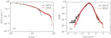
The turbulent kinetic energy spectrum and the probability density function (PDF) of velocity gradient tensor are important in analyzing the multi-scale features of any turbulent flows. These two parameters obtained by LES and DNS are compared for the polymer solution case, as shown in Fig. 1. Because of the isotropy of FHIT, only PDF of the velocity gradient tensor in the x direction is given. It is shown that the turbulent kinetic energy spectrum and PDF of ∂ u/∂ x obtained from the LES results coincide well with the corresponding DNS results, which on one hand demonstrates the correctness of the LES code based on MCT SGS model for FHIT in the polymer solution. Note that, due to the limitation of the simulated grid number in LES (323) and the truncated turbulence scale, the resolved wavenumber k cannot reach the high value corresponding to the dissipation scale as obtained in DNS (963), so that the plateau-like structure in E(k) profile of polymer solution case obtained by DNS as shown in Fig. 1(a) (which was reported in our previous DNS study of decaying homogeneous isotropic turbulence[19]) cannot be captured in the current LESs based on MCT.
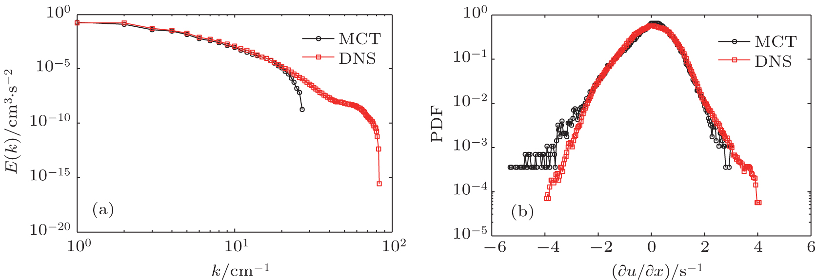 | Fig. 1. (a) Turbulent kinetic energy spectrum; (b) PDF of ∂ u/∂ x for the viscoelastic fluid flow at Wi = 0.34, β = 0.8. |
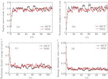
When turbulence comes into a statistically stable state in FHIT, some statistically stationary turbulent quantities, such as the Taylor micro-scale 
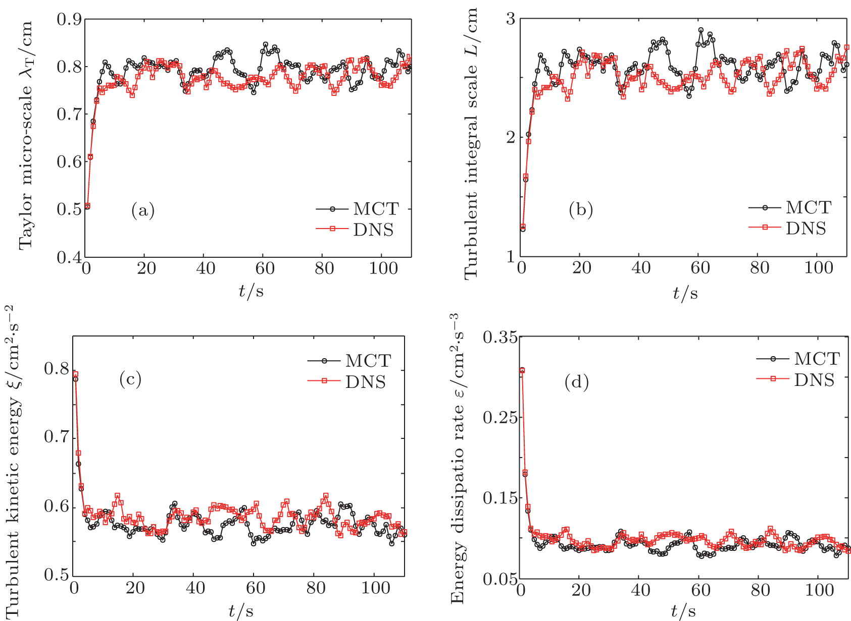 | Fig. 2. Four turbulent basic parameters for the viscoelastic fluid flow at Wi = 0.34, β = 0.8. (a) Taylor micro-scale; (b) turbulent integral scale; (c) turbulent kinetic energy; (d) energy dissipation rate. |
| Table 3. Statistically stationary turbulent quantities for LES and DNS in the Newtonian fluid and viscoelastic fluid. |
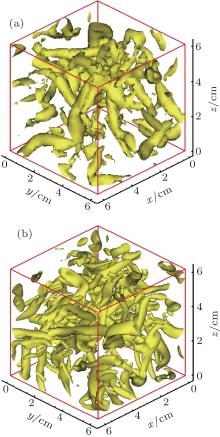
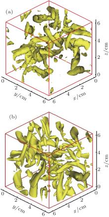
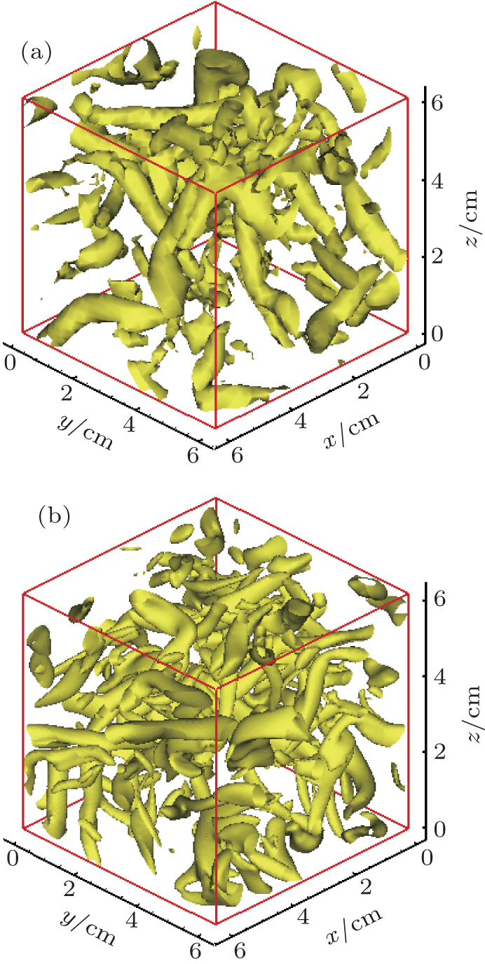
In this study, the MCT model makes use of the idea related with the Q method defined for extracting CSs in turbulence. The positive Q signifies a vortex tube, which can give rise to the intermittency of turbulence. Extraction of CSs for turbulent flows, including homogeneous isotropic turbulence and wall-bounded turbulent flows, has been of great help in investigating the characteristics of turbulence.[59– 62] Research on the variation of vortex tubes in FHIT influenced by polymer additives is significant for exploring the mechanism of turbulent DR in turbulent drag-reduced flows. In order to further validate the MCT model and the LES code, comparisons of turbulent vortex tubes based on LES and DNS databases have been carried out for the Newtonian fluid and polymer solution cases, as shown in Figs. 3 and 4, respectively. (Here, figure 3 is for the Newtonian fluid case, which serves in the role of the comparative object to illustrate the effect of drag-reducing additives on vortex tubes.) It can be seen that the vortex tubes extracted from the LES database are not as smooth as those from the DNS result, which is caused by the coarse grid number (323) used for LES as compared with the grid number 963 used for DNS. It is also reasonable that the quantity of the extracted vortex tubes in FHIT of the Newtonian fluid and viscoelastic fluid by LES is less than that by DNS at the same conditions, which is obviously caused by the nature of turbulence-scale truncation performed by LES. Regardless of the above factors, the study shows that the characteristics of vortex tubes in LES and DNS results are similar to some extent, and importantly, LES as well as DNS can resolve the salient phenomenon in FHIT affected by drag-reducing additives: the quantity of vortex tubes decreases in viscoelastic fluid flow compared with that in the Newtonian fluid flow (comparing Fig. 3(a) with Fig. 4(a) for LES, and Fig. 3(b) with Fig. 4(b) for DNS). Therefore, the results obtained by our LES code based on MCT are correct from the viewpoint of extracting vortex tubes as well, which validates one more time our LES code for simulating FHIT in polymer solution.
 | Fig. 3. The Q = 3 isosurfaces for extracting vortex tube structures for the Newtonian fluid at t = 80 s, based on (a) CSM and (b) DNS. |
 | Fig. 4. The Q = 3 isosurfaces for extracting vortex tube structures for the viscoelastic fluid at t = 80 s, based on (a) MCT and (b) DNS. |
First, an overview of our DNS results for turbulent channel flows with surfactant additives is presented and some comparisons between our DNS results (D1 in Table 2) with the published data by Yu and Kawaguchi[13] are also performed. Our DNS results for the case D1 are obtained in a 64 × 64 × 64 grid system with Δ x+ = 23.4 and Δ z+ = 11.7 in the streamwise and spanwise directions, respectively, and 0.45 ≤ Δ y+ ≤ 9 in the wall-normal direction, which is the same as those in Ref. [13]. For the viscoelastic fluid case, we obtain 41.5% DR, 〈 U+ 〉 = 23.9 at the channel centerline and 〈 − u+ ′ v+ ′ 〉 = 0.56 at y+ ∼ 37.9 for the D1 case, which are all close to those obtained by Yu and Kawaguchi, [13] i.e., DR = 42.8%, 〈 U+ 〉 = 24.1 at the channel centerline and 〈 − u+ ′ v+ ′ 〉 = 0.55 at y+ ∼ 37.9 (see Table 2, Figs. 3(a) and 3(b) in Ref. [13]). By the above mentioned comparisons, it is proved that our DNS results are correct and can be used as the benchmark for verifying the MCT SGS model.
Then the validation of our in-house LES codes for turbulent drag-reducing channel flows based on MCT SGS model is performed by comparing LES results with the corresponding DNS results. For surfactant solution flows, the two cases at Weτ = 25, β = 0.8, and Weτ = 40, β = 0.8 at Reτ = 180 (D2, D3, M1, and M2 in Table 2) are chosen from all the simulated cases as the representative examples used for comparison.
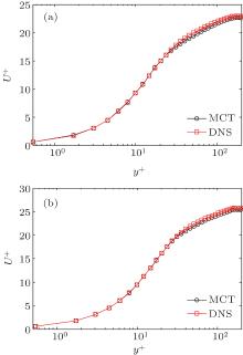
Figure 5 shows profiles of the non-dimensional streamwise velocity obtained by LES based on the MCT model and DNS, respectively. It is clearly seen that profiles of the mean velocities by LES using MCT SGS model agree quite well with those by DNS for the two cases. Only a small discrepancy exists: the MCT SGS model slightly underestimates the mean velocity in the logarithmic layer as compared with DNS. Since the CSM SGS model, which is adopted to filter the momentum equation in the present MCT SGS model, slightly overestimates the mean velocity of the Newtonian fluid turbulent channel flow in the verification of CSM, [28] the underestimated phenomenon shown in Fig. 5 could be influenced by the addition of the conformation tensor transport equation.
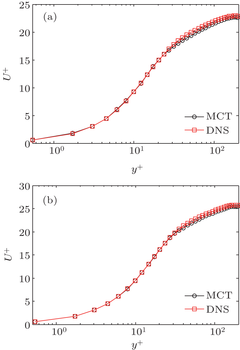 | Fig. 5. Distribution of non-dimensional mean velocity with y+ for viscoelastic fluid at (a) Weτ = 25, β = 0.8; (b) Weτ = 40, β = 0.8. |
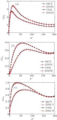
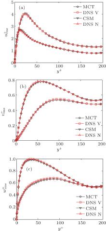
In order to better verify the MCT SGS model, the comparison of pulsating quantity is essential. Turbulent intensities are typical pulsating quantities for turbulent channel flow, and the comparative results are shown in Figs. 6 and 7 for the two selected viscoelastic fluid cases and their Newtonian fluid counterpart, respectively. It is shown that the profiles of all components of the turbulent intensities by LES using the MCT SGS model are in good agreement with those by DNS. All the typical phenomena appeared in the profiles of turbulent intensities for a drag-reduced turbulent flow by additives have been excellently resolved: the peaky positions of the streamwise, wall-normal and spanwise velocity fluctuations in viscoelastic fluid move far away from the wall as compared to those for the Newtonian fluid case; the peak-value of the streamwise velocity fluctuation (normalized with the friction velocity) in viscoelastic fluid is higher than that in the Newtonian fluid, while the wall-normal and spanwise velocity fluctuations are all decreased (as clearly shown in Figs. 6 and 7). This demonstrates that the currently proposed MCT SGS model is able to accurately describe the turbulent pulsating quantities in a drag-reduced turbulent flow of viscoelastic fluid.
 | Fig. 6. Normalized velocity fluctuation intensities (“ N” and “ V” represent the Newtonian fluid and viscoelastic fluid at Weτ = 25, β = 0.8, respectively). (a)    |
 | Fig. 7. Normalized velocity fluctuation intensities (“ N” and “ V” represent the Newtonian fluid and viscoelastic fluid at Weτ = 40, β = 0.8, respectively). (a)    |
It has been well documented that the flow resistance in a turbulent channel flow can be greatly decreased by the addition of drag-reducing polymer/surfactant additives, leading to DR, [5– 10, 45, 63] and the Reynolds shear stress has a direct quantitative relationship with the turbulent contribution to the friction factor in a wall-bounded turbulent flow.[64] Therefore, the quantitative prediction of the Reynolds shear stress is of crucial significance for turbulent channel flow with drag-reducing additives. Figure 8 plots the distributions of the Reynolds shear stress obtained by LES based on the MCT SGS model as compared with that obtained by DNS, showing quite good agreement. And the salient feature appearing in the profile of the Reynolds shear stress for a turbulent drag-reduced flow by additives is captured: the Reynolds shear stress is greatly decreased, particularly in the buffer layer region, by the additives, as compared with the Newtonian fluid counterpart. This indicates on one hand that the MCT SGS model is capable of precisely capturing the flow resistance in a turbulent channel flow with drag-reducing additives.
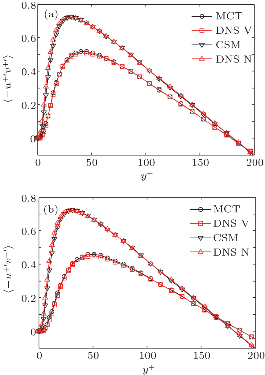 | Fig. 8. Distributions of the Reynolds shear stress with y+ for viscoelastic fluid cases at (a) Weτ = 25, β = 0.8; (b) Weτ = 40, β = 0.8 (“ N” and “ V” represent the Newtonian fluid and viscoelastic fluid, respectively). |
The DR rate for a turbulent drag-reducing channel flow by additives is defined as
where 


| Table 4. Friction factors and DR rate. |
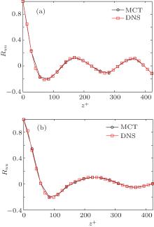
Figure 9 shows profiles of the autocorrelation coefficient of the streamwise velocity component Ruu in the spanwise direction, which reflects a quantitative measure of the spanwise distance between two neighboring near-wall low-speed streaks in a wall-bounded turbulent flow: the corresponding spanwise distance at the first peaky structure of Ruu profile is approximately the spanwise separation spacing between two neighboring low-speed streaks. Again, quite good agreements of the Ruu profiles between the results obtained by LES based on MCT SGS model and those by DNS can be observed. Due to the coarse grid used for LES, the location of the minimum Ruu obtained by LES deviates slightly from that obtained by DNS. With the increase of the Weissenberg number, the spanwise separation spacing of the near-wall low-speed streaks is increased, indicating a weakening effect of the turbulent bursting event by the drag-reducing additives.
 | Fig. 9. Two-point spanwise correlations of the velocity component in the streamwise direction at y+ = 6 for viscoelastic fluid at (a)Weτ = 25, β = 0.8; (b)Weτ = 40, β = 0.8. |
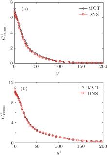
In a turbulent flow of drag-reducing surfactant solution, the viscoelasticity in the flow is generated with the stretching of the microstructures formed by surfactant molecules (micelles), and the stretching strength can be reflected by the conformation fluctuation intensity. Figures 10 and 11 show profiles of the root-mean-square of the conformation fluctuations 


 | Fig. 10. Distributions of root-mean-square fluctuations for conformation component  |
 | Fig. 11. Distributions of root-mean-square fluctuations for conformation component  |
In the preceding subsection, validations of our LES code based on the MCT SGS model for viscoelastic fluid turbulent flows were elaborated. As a new SGS model particularly designed for turbulent drag-reducing flow, MCT has many advantages stemming from the spatial and temporal filtering procedures. In order to explore the typical features of the MCT model, the LES results based on MCT for FHIT in a viscoelastic fluid and drag-reduced turbulent channel flow are further discussed below.
For MCT, since the filtering approach for CSM is used to filter the momentum equation, the merits of CSM are naturally imparted into MCT. One of the advantages is that the parameter C is locally determined as shown by Eq. (3). Figures 12 and 13 show the instantaneous FCS and C at each grid cell along the centerline in the x direction and the time evolutions of FCS and C at the center point for the case V5 in Table 1 at Wi = 0.34 and β = 0.8 for FHIT with polymer additives, respectively. The model parameter C can be easily acquired by the second invariants Q and E, which are calculated from the partial derivatives of the velocity field. Since the positive Q is used for extracting CSs and has relationships with the SGS energy dissipation, it indicates that C is indirectly related to the energy dissipation. Meanwhile, C is computed dynamically, i.e., different values of C can be obtained on different grid nodes at every time step, as shown in Figs. 12 and 13. As a result, C can indirectly but exactly reflect the energy dissipation in a turbulent flow at different locations and times, unlike 
 | Fig. 12. FCS (a) and C (b) for each grid at t = 80 s based on MCT for FHIT in a viscoelastic fluid. |
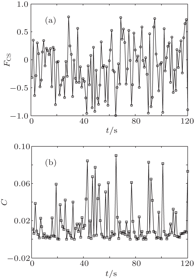 | Fig. 13. The time evolutions of FCS (a) and C (b) based on MCT for FHIT in a viscoelastic fluid. |
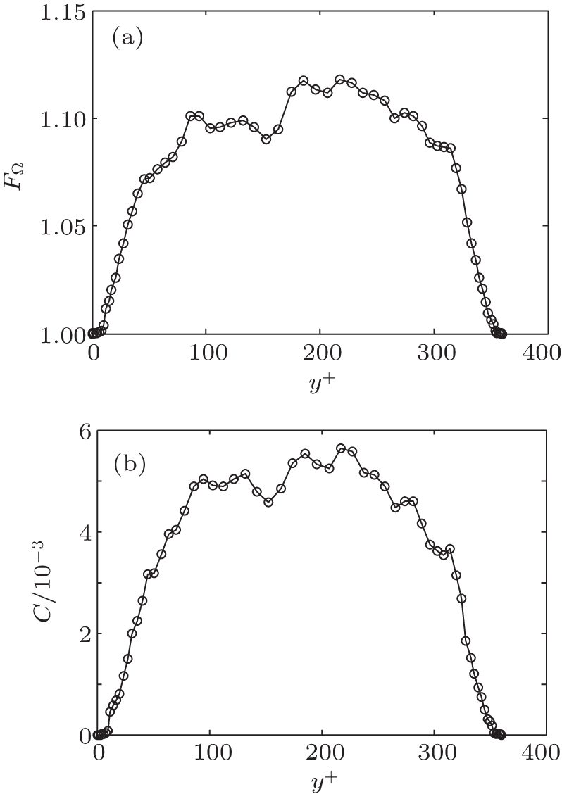 | Fig. 14. Distributions of FΩ (a) and C (b) with y+ at Weτ = 25, β = 0.8 by LES based on MCT SGS model for viscoelastic fluid in a turbulent channel flow. |
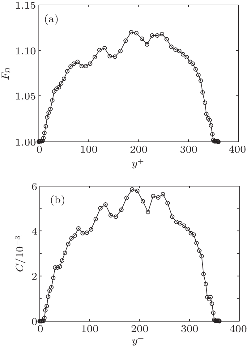 | Fig. 15. Distributions of FΩ (a) and C (b) with y+ at Weτ = 40, β = 0.8 by LES based on MCT SGS model for viscoelastic fluid in a turbulent channel flow. |
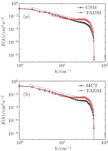
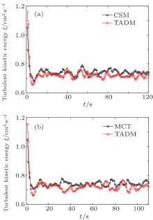
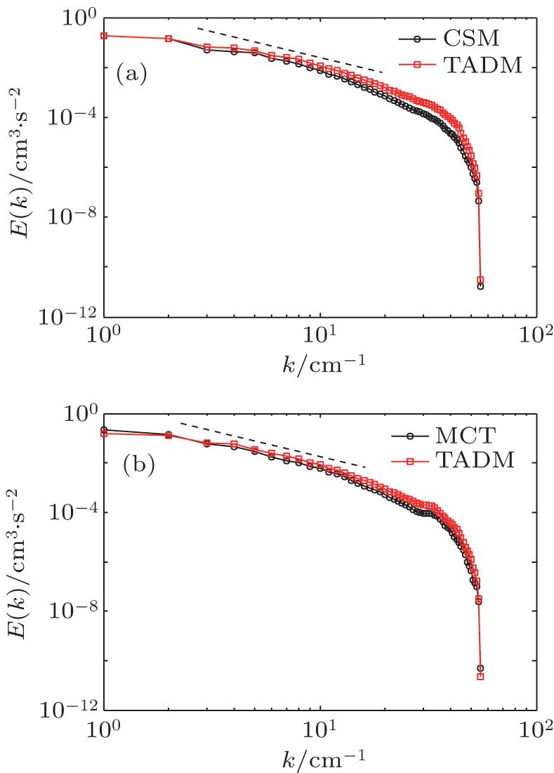
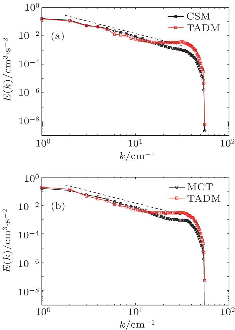
To gain further insights into the typical merits of MCT, comparisons between LES results for FHIT in viscoelastic fluid based on MCT and TADM SGS models, respectively, are presented as follows. Figures 16 and 17 plot the turbulent energy spectra for the Newtonian fluid and viscoelastic fluid cases based on CSM, MCT and TADM SGS models for Runs N1– N4 and V1– V4 (as listed in Table 1) at the same Reynolds numbers (Re = 333 and 1000), respectively. Figure 16 shows that at a relatively small Re (Re = 333), the turbulent energy spectra obtained by CSM, MCT and TADM models are similar to each other and close to the Kolmogorov theory E(k) ∼ k− 5/3 within the inertial range. This indicates that both MCT and TADM perform quite well in simulating FHIT with polymer additives at relatively small Re. Figure 17 shows that at relatively large Re (Re = 1000), the turbulent energy spectra obtained by CSM and MCT models are in accordance with the Kolmogorov theory E(k) ∼ k− 5/3 within the inertial range. However, the energy spectra obtained by TADM in the Newtonian fluid and polymer solution of FHITs are apparently deviated from the Kolmogorov theory E(k) ∼ k− 5/3 in a range of k = 15– 35. In order to explore this phenomenon, time evolutions of the turbulent kinetic energy and energy dissipation rate for the Newtonian fluid and viscoelastic fluid are given in Figs. 18 and 19. We can see that the turbulent kinetic energy for MCT and TADM are essentially the same, but the energy dissipation rate for TADM is obviously higher than that for MCT. This means that the dissipated energy in FHIT is overestimated by the TADM SGS model, resulting in the deviated energy spectrum for TADM at Re = 1000, even for the Newtonian fluid case. This indicates that LES based on the TADM SGS model does not correctly predict the turbulent energy dissipation rate at relatively high Re, while that based on MCT model does. Therefore, it can be concluded that the newly proposed MCT SGS model is superior to TADM in LES of high-Re turbulent flows of viscoelastic fluids. This is important to the applications of LES in academic research, where one hopes the Reynolds number to be as high as possible and in engineering applications, where the Reynolds number is always very high.
 | Fig. 16. Turbulent energy spectrum for (a) the Newtonian fluid case and (b) λ = 0.05, β = 0.8 in viscoelastic fluid at Re = 333 (the dotted line represents the Kolmogorov hypothesis E(k) ∼ k− 5/3). |
 | Fig. 17. Turbulent energy spectrum for (a) the Newtonian fluid case and (b) λ = 0.1, β = 0.9 in viscoelastic fluid at Re = 1000 (the dotted line represents the Kolmogorov hypothesis E(k) ∼ k− 5/3). |
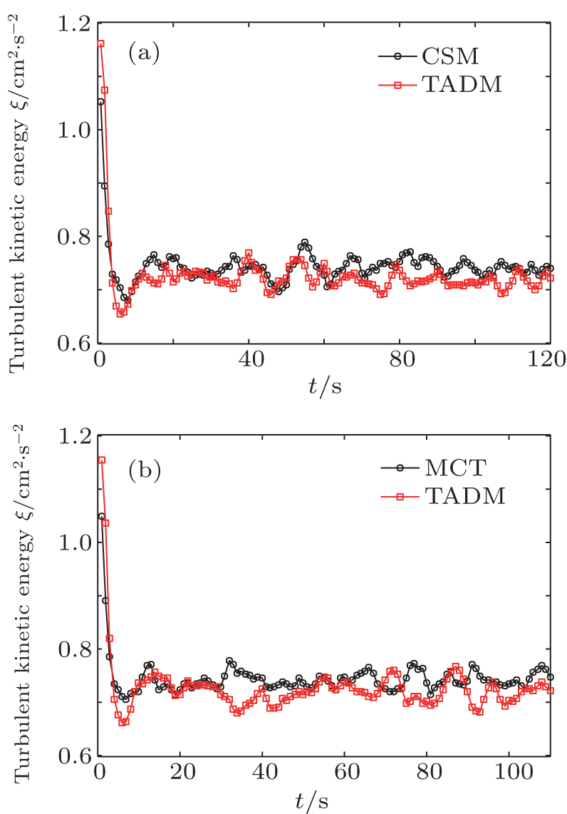 | Fig. 18. Turbulent kinetic energy for (a) the Newtonian fluid case and (b) λ = 0.1, β = 0.9 in viscoelastic fluid at Re = 1000. |
 | Fig. 19. Energy dissipation rate for (a) the Newtonian fluid case and (b) λ = 0.1, β = 0.9 in viscoelastic fluid at Re = 1000. |
A novel SGS model named MCT, particularly for LES of turbulent drag-reducing flows of viscoelastic fluids, has been proposed, which combines the ideas of CSM with spatial filtering and TADM with temporal filtering. The essence of MCT is to use CSM to filter the momentum equation with an additional subfilter term in the space domain and apply TADM to filter the conformation tensor transport equation in the time domain. The MCT SGS model can be easily realized for the LES of turbulent flows of viscoelastic fluids because only the partial derivatives of velocity field are needed to filter the momentum equation, and the filtering of conformation tensor transport equation can be obtained only by utilizing the information before and at subsequent time steps.
In order to validate the correctness of the MCT SGS model, FHIT and turbulent channel flow of viscoelastic fluids are selected as prototype turbulent flows to perform LES. The present LES results of the turbulent energy spectrum, PDF of ∂ u/∂ x, statistically stationary turbulent quantities and turbulent vortex structures for FHIT with polymer additives, as well as the mean velocity, velocity fluctuation intensities, Reynolds shear stress, friction factor, DR rate, two-point spanwise correlation and fluctuation intensities of conformation tensor components for turbulent channel flow with drag-reducing surfactant additives are all compared with those of the corresponding DNS results. From the comparative consequences, it is manifest that the above parameters obtained from LES based on the MCT model are all in quite good agreement with those from DNS, indicating the correctness of our LES codes and the newly proposed MCT SGS model. So the features of MCT have been explored from several aspects. The locally determined model parameter C for MCT has a relationship with the energy dissipation in turbulent flows, and so it correctly reflects the turbulent energy dissipation at every time step and every grid cell. Furthermore, C is always positive due to its upper and lower limits, ensuring the steadiness of the numerical simulation process. By comparing the LES results based on the MCT and TADM SGS models, respectively, for polymer solution cases, at the same conditions, it is obtained that LES based on the TADM model fails to correctly simulate FHIT in both the Newtonian fluid and viscoelastic fluid at relatively large Reynolds numbers, but when based on MCT, it succeeds. Therefore, this new mixed SGS model MCT designed particularly for LES of turbulent flow of viscoelastic fluid shows superior potential in solving both academic problems and engineering application issues about turbulent drag-reducing flows at high Reynolds numbers.
| 1 |
|
| 2 |
|
| 3 |
|
| 4 |
|
| 5 |
|
| 6 |
|
| 7 |
|
| 8 |
|
| 9 |
|
| 10 |
|
| 11 |
|
| 12 |
|
| 13 |
|
| 14 |
|
| 15 |
|
| 16 |
|
| 17 |
|
| 18 |
|
| 19 |
|
| 20 |
|
| 21 |
|
| 22 |
|
| 23 |
|
| 24 |
|
| 25 |
|
| 26 |
|
| 27 |
|
| 28 |
|
| 29 |
|
| 30 |
|
| 31 |
|
| 32 |
|
| 33 |
|
| 34 |
|
| 35 |
|
| 36 |
|
| 37 |
|
| 38 |
|
| 39 |
|
| 40 |
|
| 41 |
|
| 42 |
|
| 43 |
|
| 44 |
|
| 45 |
|
| 46 |
|
| 47 |
|
| 48 |
|
| 49 |
|
| 50 |
|
| 51 |
|
| 52 |
|
| 53 |
|
| 54 |
|
| 55 |
|
| 56 |
|
| 57 |
|
| 58 |
|
| 59 |
|
| 60 |
|
| 61 |
|
| 62 |
|
| 63 |
|
| 64 |
|