


Effects of evacuation assistant’s leading behavior on the evacuation efficiency: Information transmission approach
[Wang Xiao-Lua) , Guo Weia) , Zheng Xiao-Ping†b)  ]
]
]
|
|


†Corresponding author. E-mail: asean@mail.tsinghua.edu.cn
*Project supported by the National Basic Research Program of China (Grant No. 2011CB706900), the National Natural Science Foundation of China (Grant Nos. 71225007 and 71203006), the National Key Technology Research and Development Program of the Ministry of Science and Technology of China (Grant No. 2012BAK13B06), the Humanities and Social Sciences Project of the Ministry of Education of China (Grant Nos. 10YJA630221 and 12YJCZH023), and the Beijing Philosophy and Social Sciences Planning Project of the Twelfth Five-Year Plan, China (Grant Nos. 12JGC090 and 12JGC098).
Evacuation assistants are expected to spread the escape route information and lead evacuees toward the exit as quickly as possible. Their leading behavior influences the evacuees’ movement directly, which is confirmed to be a decisive factor of the evacuation efficiency. The transmission process of escape information and its function on the evacuees’ movement are accurately presented by the proposed extended dynamic communication field model. For evacuation assistants and evacuees, their sensitivity parameter of static floor field (SFF),
During emergency evacuation, well-trained evacuation assistants (EAs) generally have global information and greater experience, and their duty is to help evacuees escape as quickly as possible. Generally, EAs can be divided into two types in terms of functions: guider and leader. The former guides evacuees by transmitting route information with respect to the exits, and the latter leads evacuees by transferring the route information concerning his own position. When the escape routes are too complex to be understood by evacuees, EAs that act as the leader can gather evacuees and lead them toward the exit together.[1] To improve their leading efficiency, EAs have to continually shout out command signals such as “ follow me” , and transmit their own position information such that evacuees can find and follow them. Then it is necessary for EAs to adjust their leading speed according to the crowd’ s collective motions. However, EAs’ personal abilities such as physical agility and event handling capability are limited. The leading efficiency is greatly influenced by the leading speed and mobilization ability of EAs, crowd’ s following speed, etc. Therefore, it is essential and significant to explore the factors that influence an EA’ s leading behavior from the perspective of information transmission.
The escape speed of the crowd directly affects the evacuation time. Based on the information transmission, the current studies mainly focus on EAs’ guiding and leading speed and related factors that influence the evacuation efficiency. Both the biology studies[2, 3] and human evacuation experiments[4, 5] have demonstrated that the information plays an important role in the route selection process of individuals. Through their experiments, Faria et al.[6] concluded that the individuals with information were able to lead the group effectively and accurately to the target and that the group position of informed individuals was indeed correlated with group performance. By modeling and simulation, Aubé and Shield[7] analyzed the effectiveness of EAs’ placement on crowd control. Mixing in different leader types, placing some in the immediate proximity of the crowd and others scattered around the environment, provides desirable results, and leaders that operate at approximately half the speed of other agents lead to the most efficient evacuations. Pelechano et al.[8] presented a “ multi-agent communication for evacuation simulation” , where an EA who has the complete route knowledge aimed to communicate with others during the evacuation. Yuan et al.[9] simulated the phenomenon of “ flow with the stream” based on the cellular automaton (CA) model and showed that the route information was indirectly shared through individuals’ tendency to follow behavior that improved the evacuation efficiency. Henein and White[10] introduced the role of force and developed the CA model to be more realistic in the aspect of describing the information communication process among individuals. Wang et al.[11] proposed the communication field (CF) model to describe the transmission and effect of escape information spread by EAs, showing how evacuees gradually increase the knowledge of unknown exit and escape routes after receiving the escape information. The result indicated that locating EAs near exits reduces the time delay for pre-evacuation. Hou et al.[12] studied the effects of the number and positions of the trained EAs in multi-exits rooms based on the SF model. The results indicated that there should be as many EAs as the number of exits, and the initial positions and responsible areas of EAs should be focused on. More and more works focus on the importance of information transmission, which is the way that EAs influence the evacuation process. However, the relationship of relative movement speed between EAs and evacuees has not attracted sufficient attention so far.
CA is a typical discrete model that is widely used in simulating pedestrian movement.[13– 17] Three methods are commonly used for describing an agent’ s speed. The first one takes advantage of the sensitivity parameter kS of the static floor field in the floor field model, which could control the effective walking speed.[18– 22] It is based on the transition probability that an agent moves from the current position to a neighboring cell per time step. For high computational efficiency of the floor field model, it is the most common application in various scenario simulations.[23, 24] The second one uses a fine division of a discrete cell.[25– 27] However, the calculation consumption is a great issue that must be considered. Furthermore, only the final state of an agent’ s movement and conflicts in the desired new positions are considered, while the intermediate positions are ignored. The third way is to divide the time scale into multiple sub-time steps; agents of different speeds asynchronously update the position in each corresponding sub-time step.[28] Through this way, the simulation time also increases due to the successive treatment of the sub-time steps, which is not suitable for large crowd evacuation simulation. In essence, the three methods all approximate the agent’ s speed. In the present work, the first description method is adopted.
For the leading efficiency of EAs, an extended dynamic communication field (DCF) model is presented to describe the transmission process of an EA’ s dynamic position information as well as the information function on evacuees that gather around and follow the EA. The effect of the EA’ s leading behavior on evacuation efficiency was examined and analyzed.
Because CA models can be used to describe the transmission and effect of information from the microscopic perspective, the CF model (based on CA) is used to describe the efficiency of an EA.[1] For the previous model, information disseminated by an EA is considered to be the shortest path from an evacuee’ s current position to the exit (represented by a static floor field that remains constant over time). However, when EAs show the leading behavior, their dynamic position information must be spread to the evacuees following them. Because an EA’ s position and leading routes change every moment during the leading process, an extended dynamic communication field (DCF) model is incorporated.
The route information field SL(i), which is time-dependent, is introduced to describe the shortest route, with the position of EA L(i) as the destination. The value of SL(i) for position (x, y) at time t, expressed as SL(i) (x, y, t), is determined by the nearest distance from any position in a scene to the EA’ s position (a, b) and is calculated by the Euclidean measure given by
The route information of the building exit E(i) is expressed as SE(i) (static floor field) to describe the shortest route, with the building exit’ s position as the destination. The complete route information for the scene S is given by

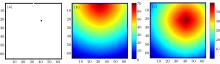
Corresponding to the scene shown in Fig. 1(a) (with an EA located in the compartment), figure 1(b) describes the value of the static floor field SE(i) and figure 1(c) describes the value of the route information field SL(i). From Fig. 1(c), one can see that the EA’ s position appears similar to an exit inside the scene, which also attracts the evacuees just as a building exit would.
In previous literatures, the value of kS, as the coupling to SFF, refers to escape motivation[10, 18, 21] or the knowledge of escape routes.[29] Here, for individuals the sensitivity parameter kSi reflects the degree of uncertainty concerning the route information Si ∈ S. For kSi → 0, the individual is entirely ignorant of Si, and thus would perform a pure random walk. In contrast, a larger kSi means that the individual knows more about Si, and for kSi → ∞ he is capable of knowing the whole escape routes and can make deterministic choices according to the shortest routes. This means that a larger kSi implies a larger average velocity of freely moving pedestrians. During the evacuation, evacuees would continually receive the information transmitted by EAs, thus causing their kSi to change dynamically. In contrast, the kSi of EAs would remain the same in an evacuation. For distinction, we use 


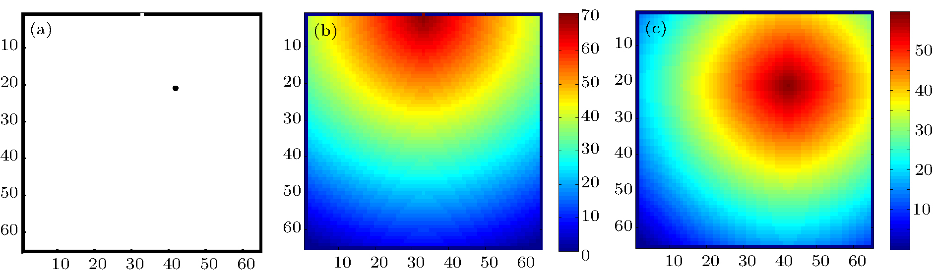 | Fig. 1. Route information field value: (a) the scene; (b) with the exit as the destination; (c) with the EA’ s position as the destination. |
Analogous to the sound propagation process, some information particles are dropped by an EA at each time step, with his position as the center and within a radius of RL(j) m which is a key factor of an EA’ s mobilization ability. At the next time step, these information particles vanish. 

Figure 2 shows the information particles’ instant picture. Figure 2(a) shows the transmission range at a fixed position, and figure 2(b) shows the transmission range during the dynamic process of an EA moving from the lower right corner to the exit. In addition, the transmission of information incorporates an EA’ s leading behavior, and the above processes constitute the complex transmission mode of information.
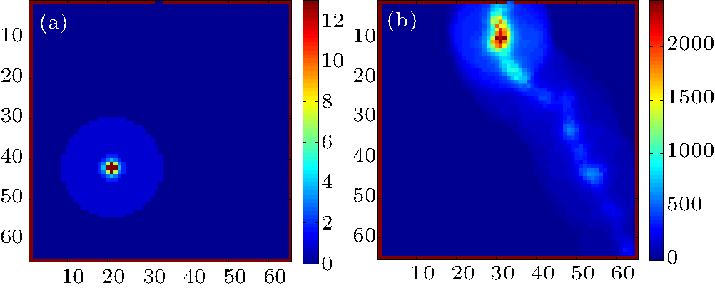 | Fig. 2. Information particles’ instant pictures: (a) the transmission range at a fixed position; (b) the transmission range during the dynamic process of an EA moving from the lower right corner to the exit. |
As long as the current location contains information particles, evacuees at that location will receive the information. The evacuees who have received information particles will comprehend relevant escape routes S according to the specific route information, and the change rate of

which is monotonically increasing. Here 
At each time step, evacuees will choose the most advantageous escape route according to their comprehension. By using the DCF model, the transition probability P that evacuees or EAs will move from their cell (x0, y0) to a neighboring cell (x, y) is expressed by


where D refers to the dynamic floor field (DFF) and kD ∈ [0, ∞ ) represents its parameter, indicating the degree of herding behavior among evacuees or EAs. Each single boson of the DFF decays with probability δ ∈ [0, 1] and diffuses with probability α ∈ [0, 1].
The proposed DCF model is applied to a single-exit compartment discretized into 65 × 65 CA cells, with two cells representing the exit. Each cell is 0.4 m × 0.4 m and can be occupied by a pedestrian or an obstacle. In the following simulations, 400 evacuees and 1 EA are assumed. When t = 0, we set 
The update rules are described as follows.
Step 1 The room and the positions of the exits, the EA and evacuees are initialized. The value of SE is calculated, and the initial value of DFF is 0.
Step 2 The value of SL is calculated. The EA drops information particles. The values of the evacuees’ DFF are updated. If an evacuee has received information particles, the value of his 
Step 3 Transition probability is calculated separately for the EA and evacuees. According to the results, target cells are chosen. More than one evacuee should choose the same target cell at the same time, then one evacuee is randomly assigned to the cell, while the rest remain in their original positions.
Step 4 Evacuees who change positions generate DFF. Information particles dropped by the EA disappear.
Step 5 Upon passing through the exit and leaving the compartment, evacuees are removed from the system. The simulation ends when all evacuees have left the compartment; otherwise, Step 2 is repeated.
For evacuees, the value of 


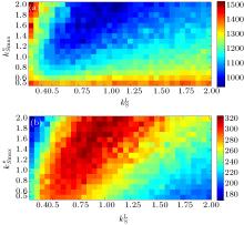
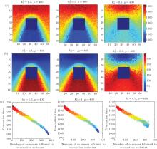
From Fig. 3(a), one can observe that the evacuation time could be less than 1100 time steps (which is relatively low in the current simulation scenario) in certain combinations of 

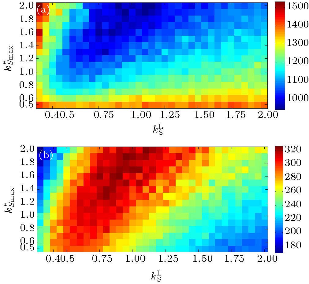 | Fig. 3. For every group comprising the EA’ s |
To analyze the evacuation processes with different 


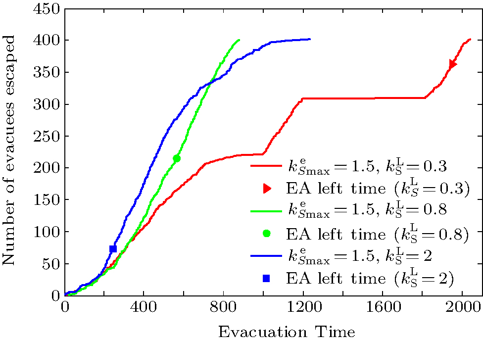 | Fig. 4. The number of evacuees that escape during three evacuation processes: |
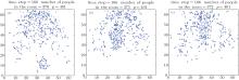
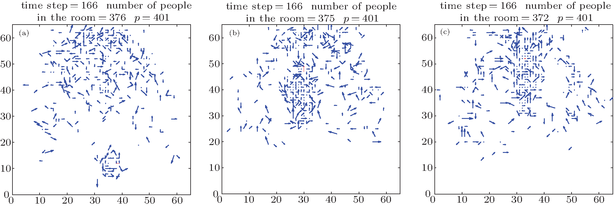 | Fig. 5. Screenshots of typical evacuation processes at the same 166th time step, corresponding to the three curves: (a) |
For further analysis on the evacuation curves, the screenshots of a few typical evacuation moments corresponding to the above three curves are shown, respectively. The velocities of evacuees are represented by blue arrow lines; the velocity of the EA is represented by a red arrow line. The velocities of the EA and evacuees are calculated by their average velocity within 5 time steps.
The screenshots of the evacuation processes at the same 166th time step, corresponding to the three curves, are shown in Figs. 5(a)– 5(c). For
Corresponding to Fig. 3(a), the contour plot for an evacuation time less than 1050 time steps is shown in Fig. 6. Two tangent lines, l1 and l2, are obtained with an intersect point at (0.5, 1), and their slopes are calculated, respectively, as kl1 = (2− 1)/(0.75− 0.5) = 4 and kl2 = (2− 1)/(1.5− 0.5) = 1. All the optimal combinations of 
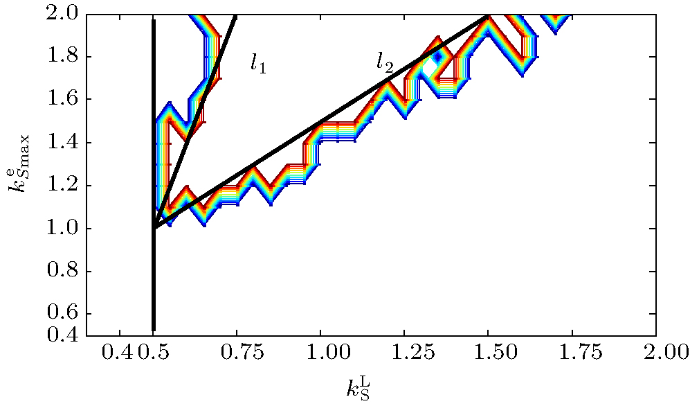 | Fig. 6. Contour plot of the evacuation time, which is less than 1050 time steps. |
Assume that the evacuees are randomly distributed in the compartment with 


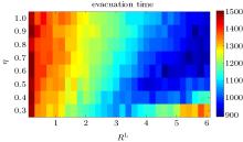
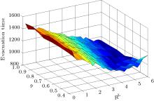
 | Fig. 7. Evacuation times for RL and η . |
| Table 1. Estimated values of each variable. |
From Fig. 7, one can see that the evacuation time could be less than 1000 time steps for certain RL and η combinations. When η ≥ 0.4, the evacuation time decreases along with RL growing large. Regression analysis is carried out on the evacuation time with RL and η . After removing the data group with η = 0.3, the evacuation times of η ≥ 0.4 are presented as the three-dimensional diagram in Fig. 8. It is found that there is a linear relationship between evacuation time and η and RL. A regression equation is assumed as 
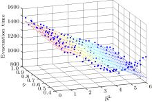
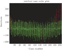
The regression plane and the data points in the three-dimensional diagram are shown in Fig. 9. Most of the data points are located in or close to the regression plane. When RL > 5 m and η < 0.6, the deviation of data points with the regression plane is large, which is presented as the upward tilt in the lower right corner of the evacuation time surface in Fig. 8. Taking the sequence number of the observed value as the horizontal coordinate and the residual error as the vertical coordinate, as shown in Fig. 10, the variation range of each observed value’ s residual error and the confidence interval are presented. The exceptional data points are marked in red. Most of the exceptional data points distribute at the end of the axis.
Looking into the regression parameters in Table 1, the coefficient of determination is R2 = 0.9013, which indicates that the regression plane could fit well with the relationship between the data. F = 945.0801 > F1− 0.05 (2, 207) = 3.00 and significance level p < 0.0001 < 0.05, which explains that there is a significant linear relationship between the independent variable and dependent variable and that the change of the independent variables can really reflect the linear change of the dependent variable. For the regression coefficients β 0 and β 1, the 95% confidence interval is narrow, which shows a high credibility of the estimated value. For the regression coefficient β 2, the confidence interval is relatively wide, which shows less credibility of the estimated value; a reason for that is the influence of the exceptional data points. By administering the t-test on the regression coefficients, the result is H = 1. Thus, the original hypothesis is rejected and it is believed that both of the regression coefficients β 0 and β 1 are significantly different from 0. This means that the two independent variables all show significant linear relationships with their respective dependent variables and should be kept in the regression equation. Thus, the relationship between evacuation time, RL, and η can be approximately expressed as

From Eq. (7) it is known that the evacuation time is shorter when RL is larger and longer when η is larger. The evacuation time should remain constant when the ratio of the increment of RL and the increment of η is approximately 75/88. However, the exceptional data points converge on η = 0.4, which indicates that the data group of η = 0.4 has a weak linear relationship with the evacuation time.
 | Fig. 8. Three-dimensional diagram of evacuation times (except the data for η = 0.3). |
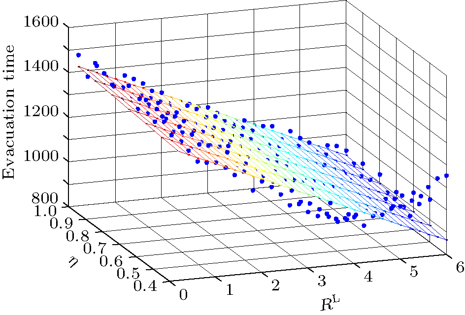 | Fig. 9. Three-dimensional diagram of the regression plane and the evacuation time data points. |
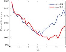
Compare the evacuation time with η = 0.3 and η = 0.4, as shown in Fig. 11. When η = 0.3, the non linear relationship is quite clear between RL and evacuation time. The optimal value of RL is 3.4 m when the evacuation time is at its lowest, which is at the 1024th time step. When η = 0.4, the evacuation time first decreases when RL increases and then rises when RL > 5 m. The optimal value of RL is 4.2 m when the evacuation time is at its lowest, which is at the 966th time step. Therefore, it is confirmed that, as η reduces from 0.4 to 0.3, the relationship between RL and the evacuation time changes from linear to nonlinear; the reason for the change can be attributed to the disturbance factors in the system. When η ≤ 0.3, the EA’ s 
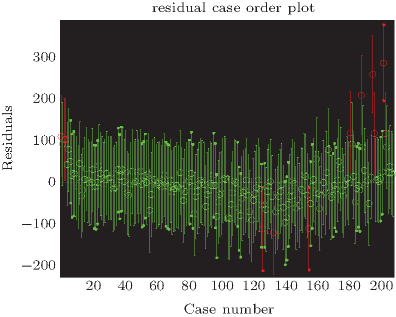 | Fig. 10. Sequential residual figure. |
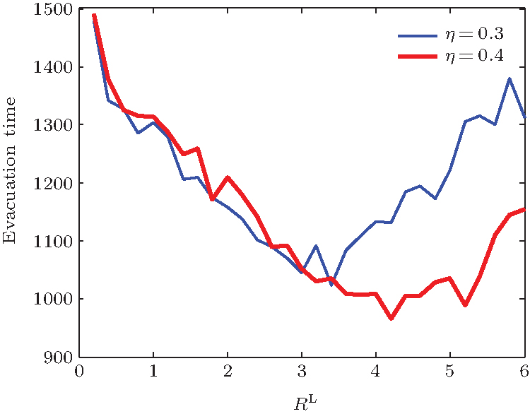 | Fig. 11. Evacuation time of two data groups: η = 0.3 and η = 0.4. |

The effect of the EA’ s 
The evacuation times of all the initial positions for the three simulation groups are shown in Fig. 12(a). The evacuation time is short when the EA’ s initial positions are in the back of the evacuee crowd and the EA can go through the crowd when he leads them to the exit (for the blue color zone). However, during the process when the EA leads them to the exit, if he only passes by the crowd from the right or left edge, then the evacuation times are longer. Even for the initial positions in front of the crowd, the evacuation times are also longer, which are shown as the green color zone. Furthermore, in the rear of the evacuee crowd, evacuation times for 

The present work aims at the model’ s theoretical analysis. When focusing on the EA’ s leading behavior and his special role during an evacuation, it is necessary to study the process by which the EAs transmit position information and the action behaviors of evacuees when they receive the information. The settings of the related parameters in the model have ensured their proper implementation above. Furthermore, the simulation results demonstrate the importance of the EA’ s leading behavior during evacuation and show that the extended DCF model is effective as an information mechanism. Through human evacuation experiments, the quantitative validation of the theoretical model could be done to help apply the model accurately. However, any human experiment conducted within a simulated emergency evacuation process needs to take into consideration the experimental risk, ethical issues, and intensive organization required, which is beyond the scope of the theoretical analysis in this paper and will be performed in our future work.
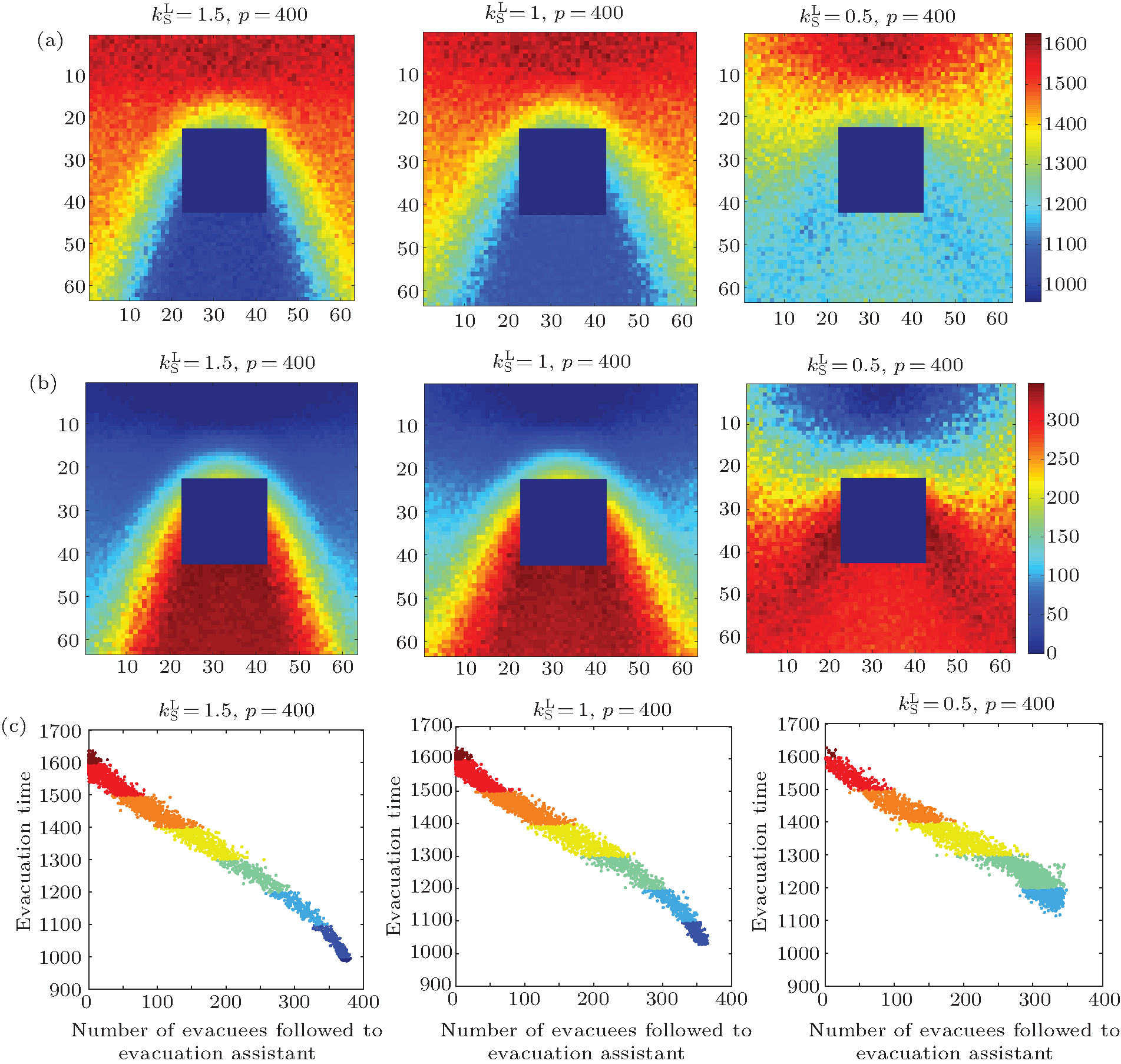 | Fig. 12. Simulation results when the evacuees’ initial position are fixed: (a) evacuation time of each initial position at three |
An extended DCF model is proposed in the present research. The transmission and function process of the escape information when an EA is moving and leading evacuees to the exit is presented. Through a large number of simulations, the relationship between the sensitivity parameters for EA’ s
i) The optimal combinations of
ii) There exists an optimal value for an EA’ s information transmission radius. When an EA’ s
iii) For the concentration distribution crowd, an EA should start at the rear of the crowd and head toward the exit, which can help in leading more evacuees and improving the evacuation efficiency.
However, in reality, individuals rely on information not only from leaders but also from their neighbours and would group together into family or friendship units. The efficiency of leaders will be influenced by such kind of social behaviors and responsibilities. In addition, the key parameters and the model have to be further verified and validated through human experiments considering leader’ s behavior. All of these above should be improved in the further work.
| 1 |
|
| 2 |
|
| 3 |
|
| 4 |
|
| 5 |
|
| 6 |
|
| 7 |
|
| 8 |
|
| 9 |
|
| 10 |
|
| 11 |
|
| 12 |
|
| 13 |
|
| 14 |
|
| 15 |
|
| 16 |
|
| 17 |
|
| 18 |
|
| 19 |
|
| 20 |
|
| 21 |
|
| 22 |
|
| 23 |
|
| 24 |
|
| 25 |
|
| 26 |
|
| 27 |
|
| 28 |
|
| 29 |
|