


An efficient locally one-dimensional finite-difference time-domain method based on the conformal scheme
[Wei Xiao-Kun†a)  , Shao Wei
a) , Shi Sheng-Binga) , Zhang Yongb) , Wang Bing-Zhonga) ]
, Shao Wei|
|


†Corresponding author. E-mail: weixiaokun1990@163.com
*Project supported by the National Natural Science Foundation of China (Grant Nos. 61331007 and 61471105).
An efficient conformal locally one-dimensional finite-difference time-domain (LOD-CFDTD) method is presented for solving two-dimensional (2D) electromagnetic (EM) scattering problems. The formulation for the 2D transverse-electric (TE) case is presented and its stability property and numerical dispersion relationship are theoretically investigated. It is shown that the introduction of irregular grids will not damage the numerical stability. Instead of the staircasing approximation, the conformal scheme is only employed to model the curve boundaries, whereas the standard Yee grids are used for the remaining regions. As the irregular grids account for a very small percentage of the total space grids, the conformal scheme has little effect on the numerical dispersion. Moreover, the proposed method, which requires fewer arithmetic operations than the alternating-direction-implicit (ADI) CFDTD method, leads to a further reduction of the CPU time. With the total-field/scattered-field (TF/SF) boundary and the perfectly matched layer (PML), the radar cross section (RCS) of two 2D structures is calculated. The numerical examples verify the accuracy and efficiency of the proposed method.
The finite-difference time-domain (FDTD) method has attracted wide attention in physical research due to its generality and simplicity.[1] It is applied in nano-techniques, [2, 3] the terahertz spectrum, [4, 5] plasma, [6, 7] photonic crystals, [8, 9] biomedical research, [10] and electromagnetic scattering.[11, 12] However, its time step is restricted by the Courant– Friedrich– Levy (CFL) condition, which leads to a long time to complete the electromagnetic (EM) simulation when tiny grids exist. To eliminate the constraint, two typical unconditionally stable time-marching methods, the alternating-direction-implicit (ADI) FDTD[13, 14] and the locally one-dimensional (LOD) FDTD, [15] were proposed. Generally, LOD-FDTD requires fewer arithmetic operations and less execution time than ADI-FDTD.[16, 17] However, although the time steps in the two methods are not limited by the CFL condition, too large time steps will lead to large numerical dispersion errors.[18, 19] To reduce their dispersion errors, some improved schemes have been introduced.[20– 22]
Besides the numerical dispersion error, there exists the staircasing approximation error when modeling curved boundaries by regular grids of FDTDs. To reduce the numerical errors generated by the staircasing approximation for curved boundary modeling, a two-dimensional (2D) nonorthogonal ADI-FDTD (ADI-NFDTD) method was proposed.[23] Furthermore, the conformal grid technique was also introduced to ADI-FDTD (ADI-CFDTD) to improve both efficiency and accuracy.[24] Based on the theoretical analysis and numerical experiments, a modified conformal technique was presented in Ref. [25] to improve the temporal stability of ADI-CFDTD. Recently, a nonorthogonal LOD-FDTD (LOD-NFDTD) method was proposed for scattering problems in the curvilinear coordinate system and high performance was achieved.[26] The LOD-NFDTD formulations for both transverse-electric (TE) and transverse-magnetic (TM) cases were derived, but its implementation was relatively complex.
In this paper, an efficient and easily implemented conformal LOD-FDTD (LOD-CFDTD) method is proposed to reduce the staircasing approximation error for solving 2D EM scattering problems. The conformal grids are only applied to the curved boundary of a metallic scatter, whereas the standard Yee grids are used in the remaining computational regions. The stability property and numerical dispersion of LOD-CFDTD are theoretically investigated. It is shown that the employment of the irregular grids does not affect the numerical stability, and the effects of the numerical dispersion from the conformal grids can be nearly neglected since the irregular grids account for a small percentage of the total space grids. The numerical stability and dispersion characteristics of the proposed technique are also checked with a numerical example of a circular waveguide, and good results are obtained. The perfectly matched layer (PML)[27, 28] is used to truncate the standard Yee lattice. And with the total-field/scattered-field (TF/SF) boundary, [29– 31] the radar cross section (RCS) of 2D structures is calculated. The numerical results show that the proposed scheme is computationally accurate and efficient compared with the traditional CFDTD and ADI-CFDTD methods.
In Section 2, updating formulations of LOD-CFDTD are presented for the 2D TE field. Then, the unconditional stability and numerical dispersion relationship are theoretically investigated and numerically verified in Sections 3 and 4, respectively. In Section 5, two numerical examples of 2D scattering problems are used to validate the proposed technique. A conclusion is presented in Section 6.
To simplify the problem, it is assumed that the wave propagates in a simple and lossless medium, the Maxwell’ s equations can be written as


where ε is the electric permittivity, and μ is the magnetic permeability.
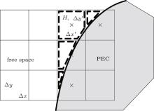
On the irregular grids intersected by a perfect electric conductor (PEC) as shown in Fig. 1, the E field is updated in exactly the same way as in the conventional LOD-FDTD method, while the H field is updated in a different way based upon Faraday’ s law along the circumference of the irregular grids. Following the derivation of LOD-FDTD’ s formulation, [15, 17] the two procedures of LOD-CFDTD that convert the explicit scheme of FDTD into the implicit one for the TEz case on the irregular grids are given as follows:sub-step 1: from time step n to n + 1/2,
 |
 |
 |
sub-step 2: from time step n + 1/2 to n + 1,
 |

 |
 |
where Δ x′ and Δ y′ are the lengths of an irregular grid outside the PEC along the x and y directions, respectively, and S is the area of the irregular grids outside the PEC. Obviously, when Δ x′ = Δ x and Δ y′ = Δ y (i.e., S = Δ xΔ y), equations (3c) and (4c) will be converted into the updating equations of H fields in the conventional 2D LOD-FDTD method.
 | Fig. 1. Cross section of a curved PEC boundary and the irregular grids. |
Since equations (3b) and (4a) cannot be calculated directly, substituting the H field equations (3c) and (4c) back to the E field equations (3b) and (4a) separately yields an implicit updating equation for the E field and an explicit updating equation for the H field at each sub-time step. The expressions of 

where

Therefore, the simultaneous linear E field equation (5) results in a tri-diagonal system that can be solved efficiently and the H field can be obtained explicitly with Eq. (3c).
Similar to the derivation of Eq. (5), the expression of Ex in the second sub-step can be obtained by substituting 

The von Neumann method is regarded as a standard technique to analyze the stability of FDTDs by evaluating the eigenvalues of amplification matrices in the spectral domain. This method has been employed to prove the unconditional stability of ADI-FDTD and LOD-FDTD, [23, 32, 33] and it is also adopted to provide evidence of the unconditional stability of the proposed LOD-CFDTD method in this paper.
For the sake of simplicity, all updating equations for field components are expressed in matrix forms. For the components to advance from time step n to n + 1/2, we have

Similarly, for the components to advance from time step n + 1/2 to n + 1, we have

where X = [Ex, Ey, Hz]T for the TEz case, and both M1 and M2 are 3 × 3 matrices that will be addressed next.
It is assumed that the spatial frequencies can be expressed by kx and ky along the x and y directions, respectively. In the spectral domain, the components at the n-th time step can be written as

where 
Substituting Eq. (8) into Eqs. (3a)– (3c), we obtain

where M1, which is the amplification matrix in the first sub-step, is expressed as

To obtain a non-trivial solution, the determinant of matrix (10) must be zero, leading to

where
The solution of Eq. (11) is given by
An equation similar to Eq. (9) for the second sub-step can be obtained by substituting Eq. (8) into Eqs. (4a)– (4c), and its solution can be derived in the same way
where

It is easy to check from Eqs. (12) and (13) that

Therefore, the proposed LOD-CFDTD is unconditionally stable and the introduction of the irregular grids does not affect its numerical stability.
Then, the unconditional stability of the proposed LOD-CFDTD method is demonstrated in an example of a 2D circular waveguide with radius 4.5 mm. The excited waveform of a Gaussian pulse is given by

where τ = 1/(2fc), t0 = 3τ , and fc = 25 GHz. The whole computational domain is divided into 24 × 24 grids and the discrete step sizes are assigned to be 0.375 mm along the x and y directions, respectively. The time step of LOD-CFDTD is defined as[24]

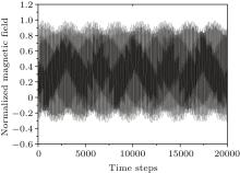
where CFLN is the time step normalized to the CFL limit of the conventional FDTD method (Δ tCFL). Unlike the conventional CFDTD method whose stability is governed by the nature of the minimum cell size and the choice of the time step, [34] the normalized H field for a long simulation time as shown in Fig. 2 demonstrates the temporal stability of the proposed method.
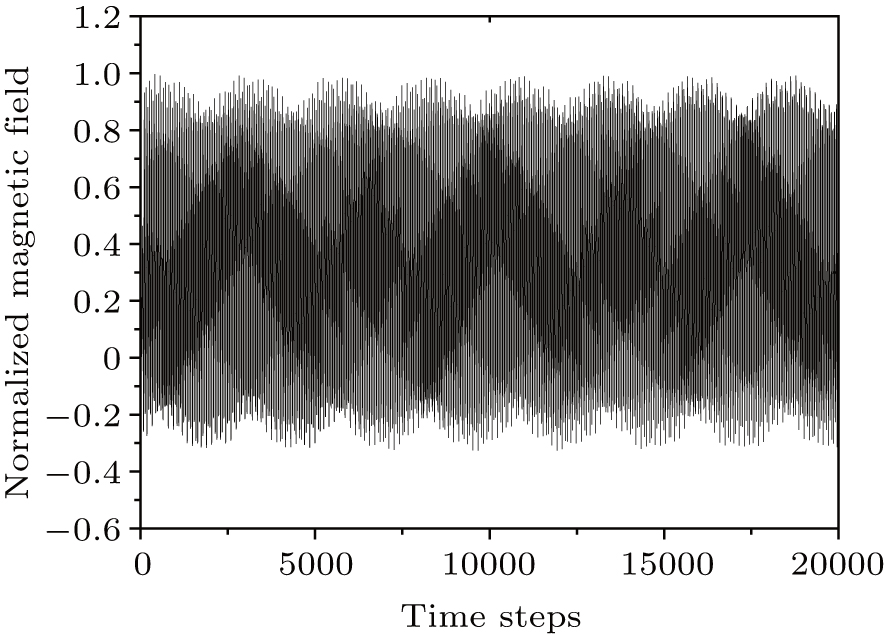 | Fig. 2. Normalized magnetic field versus time steps at CFLN = 5 using the LOD-CFDTD method. |
The finite-difference methods inevitably result in numerical dispersion errors. For LOD-CFDTD, its numerical dispersion relation is derived by applying the spectral domain technique to the field components in both sub-steps.[23, 26]
To begin with, the trial solution of the fields is assumed to be a monochromatic wave with angular frequency ω

Inserting Eq. (17) into Eqs. (3a)– (3c) gives
 |
 |
 |
Similarly, by substituting Eq. (17) into Eqs. (4a)– (4c), we obtain
 |
 |
 |
Combining Eqs. (18) and (19), we obtain
 |
 |
 |
Finally, the matrix form of Eq. (20) can be expressed as M · X = 0 and M is given by
where
By putting the determinant of matrix M to zero, the numerical dispersion relationship can be obtained as follows:

Actually, it can be observed from Eq. (22) that the numerical dispersion relationship of the proposed LOD-CFDTD method is related to three factors: the grid structure, the value of CFLN, and the number of points per wavelength (PPW). To begin with, the closer the ratios of Δ y′ /S and Δ x′ /S in an irregular grid are to 1/Δ x and 1/Δ y, respectively, the better the numerical dispersion is. It is worth mentioning that equation (22) will be converted into the numerical dispersion of LOD-FDTD in regular grid when Δ x′ = Δ x and Δ y′ = Δ y. The other two factors, CFLN and PPW, affect the numerical dispersion. Larger temporal and spatial steps introduce more dispersive errors. Obviously, as Δ t, Δ x, and Δ y tend to zero, equation (22) will be converted into the ideal dispersion relation

where k = ω /c is the theoretical wave number and c is the speed of light in free space.
There exists the staircasing approximation error when modeling curved boundaries using LOD-FDTD. In this paper, an efficient and easily implemented LOD-CFDTD method is presented to reduce the staircasing approximation error without consuming extra computer resources.
Although the LOD-CFDTD method is unconditionally stable, the accuracy of the numerical results evidently gets worse as the time step increases because of the numerical dispersion error, the same as that of LOD-FDTD.[19, 35] The effect of the conformal scheme on the numerical dispersion of the proposed method is analyzed with a numerical example below.
Now reconsider the irregular grids intersected by a PEC boundary as shown in Fig. 1, three typical cases of the area occupied by a PEC in an irregular grid are plotted in Fig. 3.
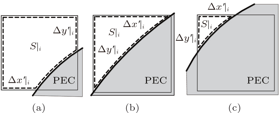 | Fig. 3. (a) A small proportion, (b) almost a half proportion, and (c) a large proportion of a Yee grid area occupied by a PEC. |
To study the effect on the numerical dispersion from different irregular grids, the ratio Ri is defined as

For simplicity, Ri is approximately assigned to be 4/7, 2, and 4 in Figs. 3(a)– 3(c), respectively. Figure 4 shows the numerical normalized phase velocity with propagation direction according to different Ri. It is a fact that the conformal scheme with different Ri has a great effect on the numerical dispersion for a single irregular grid compared to that of the regular one which can be treated as the reference, as shown in Fig. 4.
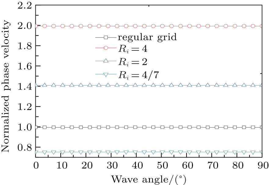 | Fig. 4. Normalized phase velocity versus the wave angle at different Ri with CFLN = 5 and PPW = 40 in LOD-CFDTD. |
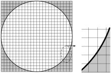
Since the conformal grids are used to model the complex region of curved boundaries only, whereas the standard Yee grids are used for the remaining regions, the irregular girds account for a small percentage of the total space grids. Here, the circular waveguide in Section 3 is employed again to validate the numerical dispersion in the whole computational region. And the grids for the whole computational region are shown in Fig. 5.
 | Fig. 5. Grids for the whole computational region of a circular waveguide. |
As shown in Fig. 5, the weighted R in the whole computational region is calculated by

where N is the total number of grids. The conformal grids account for about 13.19% of the whole grids and R is approximately equal to 0.9982 for the circular waveguide.
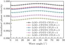
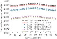
The normalized phase velocity with propagation direction of LOD-FDTD and LOD-CFDTD is shown in Figs. 6 and 7. Although the conformal scheme has a great effect on the numerical dispersion of a single grid, a small percentage of irregular grids contributes little effect to the numerical dispersion in the whole computational region. Thus the normalized phase velocity curves of the two methods only have a little difference with the same PPWs and CFLNs. Furthermore, the numerical dispersion error will be improved by increasing PPW or reducing CFLN. It can be seen from Figs. 6 and 7 that the normalized phase velocities obtained from both LOD-FDTD and LOD-CFDTD with CFLN = 1 and PPW = 40 are much closer to the ideal solution, which is a constant of 1 for all of the angles.
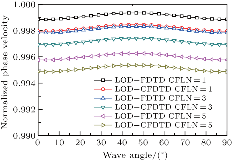 | Fig. 6. Normalized phase velocity versus the wave angle from LOD-FDTD and LOD-CFDTD with PPW = 40 at different CFLNs. |
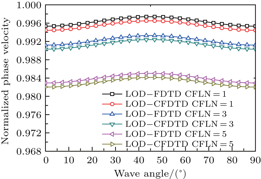 | Fig. 7. Normalized phase velocity versus the wave angle from LOD-FDTD and LOD-CFDTD with PPW = 20 at different CFLNs. |
Actually, the introduction of the conformal scheme will worsen the numerical dispersion slightly. However, it has been proved that the conformal scheme has little effect on the numerical dispersion and the effect can be nearly neglected. The introduction of the conformal scheme is to reduce the staircasing approximation error when modeling curved boundaries. Thus, it can maintain the acceptable accuracy with low PPW and improved efficiency. To validate the accuracy of the proposed method for different PPWs and CFLNs, the cutoff frequency of the TE11 mode is calculated for the circular waveguide. Figure 8 shows the relative errors obtained by LOD-FDTD using staircasing approximation and LOD-CFDTD with PPW = 20 and 40 at different CFLNs. It can be seen that the results obtained from the proposed LOD-CFDTD method are more accurate than those of the staircase approximation scheme with the same PPW. And the high PPW leads to the accurate results.
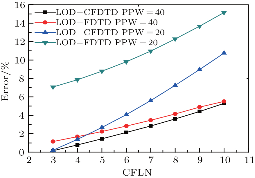 | Fig. 8. Temporal discretization convergence curves of the LOD-FDTD and LOD-CFDTD for the 2D PEC circular waveguide. |
In order to validate the proposed LOD-CFDTD method, two 2D EM scattering examples are presented in this section. The TF/SF boundary and PML are employed for the simulation of the scattering problems. Here, the results obtained from both the CFDTD and ADI-CFDTD methods are also shown for comparison. All calculations in this paper have been performed on an AMD Phenom II× 4 3.0 GHz machine with 4 GB RAM.
The surface equation of a 2D PEC superquadric cylinder is given by[23]

For γ = 2, an ellipse or a circle if a = b can be obtained. As γ → ∞ , we have a rectangle or a square if a = b.
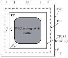
Here, a superquadric cylinder shown in Fig. 9 with γ = 4 and a = b = 2λ is considered as the first example to validate the feasibility of the proposed method. The uniform cells are used to discretize the whole computational domain, and Δ x and Δ y are chosen to be λ /40, while the conformal grids are employed to model the curved region of the superquadric cylinder scatter. The conformal grids account for only 0.34% of the grids in the whole computational domain.
 | Fig. 9. Cross section of a 2D PEC superquadric cylinder scatter and the computational domain. |
The excited waveform is given by

where τ = 1/(2fc), t0 = 3τ , fc = 1 GHz, and the incident wave is introduced in the TF/SF boundary with φ i = 0° . We choose time-marching steps of 2000 for the CFDTD method, and only 667 time-marching steps can be enough for the ADI-CFDTD and LOD-CFDTD methods when CFLN = 3.
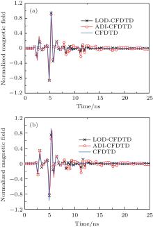
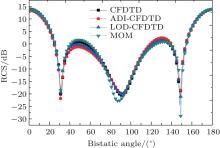
Figure 10 plots the time-domain wave curves at two different points obtained from the CFDTD, ADI-CFDTD, and LOD-CFDTD methods, and both observation points in the total field and the scattered field are five grids away from the TF/SF boundary. The far fields to calculate the bistatic RCS are 30λ away from the near-to-far-field extrapolated boundary (EB), as shown in Fig. 9. Figure 11 plots the bistatic RCS for the 2D PEC superquadric cylinder obtained from the three methods. From the two figures, it is observed that the results from the three methods agree well. Table 1 shows the computational resources involved in this example. From Table 1, it can be observed that, with the same number of grids, the LOD-CFDTD method needs less CPU time than the CFDTD and ADI-CFDTD methods when CFLN = 3.
| Table 1. Comparison of computer resources for the PEC superquadric cylinder using CFDTD, ADI-CFDTD, and LOD-CFDTD. |
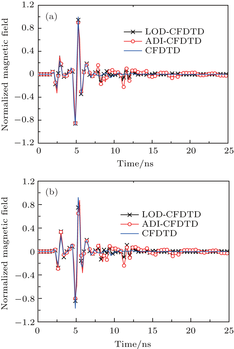 | Fig. 10. Normalized transient magnetic fields of the z component (a) at P1 (total-field) and (b) at P2 (scattered-field) obtained from the three methods. |
 | Fig. 11. Bistatic RCS of the perfectly conducting superquadric cylinder obtained from four methods. |
The scattering by two PEC elliptic cylinders which are infinitely long in the z direction is computed in the second example. Figure 12 displays the configuration of the two structures, where a = λ /10, b = 2λ , and the distance between the two elliptic cylinders is s = 0.3λ . It is very desirable that the curved outline can be well modeled using conformal grids, meaning that the computation time and memory requirement can be saved dramatically compared to the staircasing approximation scheme. The excited waveform is obtained by employing Eq. (27) again, in which fc = 1 GHz, and the incident wave is also introduced in the TF/SF boundary with the incident angle φ i = 0° . The whole computational region is 1.6λ × 4λ and will be meshed into 160 × 160 grids while the number of conformal grids accounts for only 0.56% of the grids in the whole computational domain. The cell size is assigned to be 3 mm and 7.5 mm along the x and y directions, respectively. A total number of 12000 time-marching steps for the conventional CFDTD method is needed to complete the simulation since the EM wave exists between two elliptic cylinder scatters until it vanishes after multiple-reflections. And CFLN is assigned to be 3.
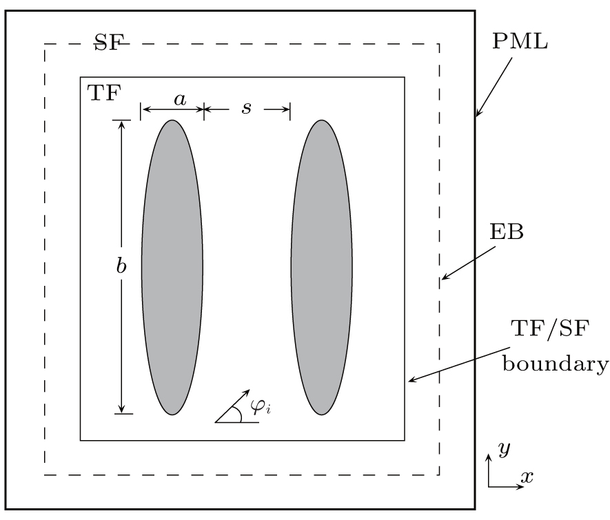 | Fig. 12. Cross section of 2D two PEC elliptic cylinders and the computational domain. |
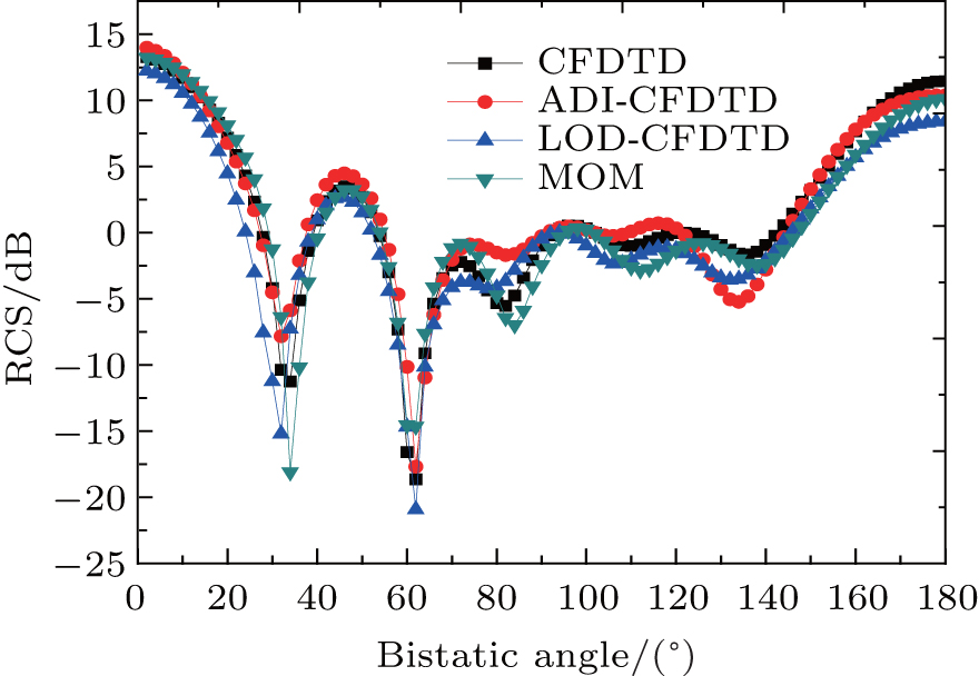
The bistatic RCS for the two 2D PEC elliptic cylinders is shown in Fig. 13. The distance for RCS calculation is also 30λ away from the EB, as shown in Fig. 12. Obviously, it can be found that the results obtained with LOD-CFDTD are in good agreement with those obtained with CFDTD.
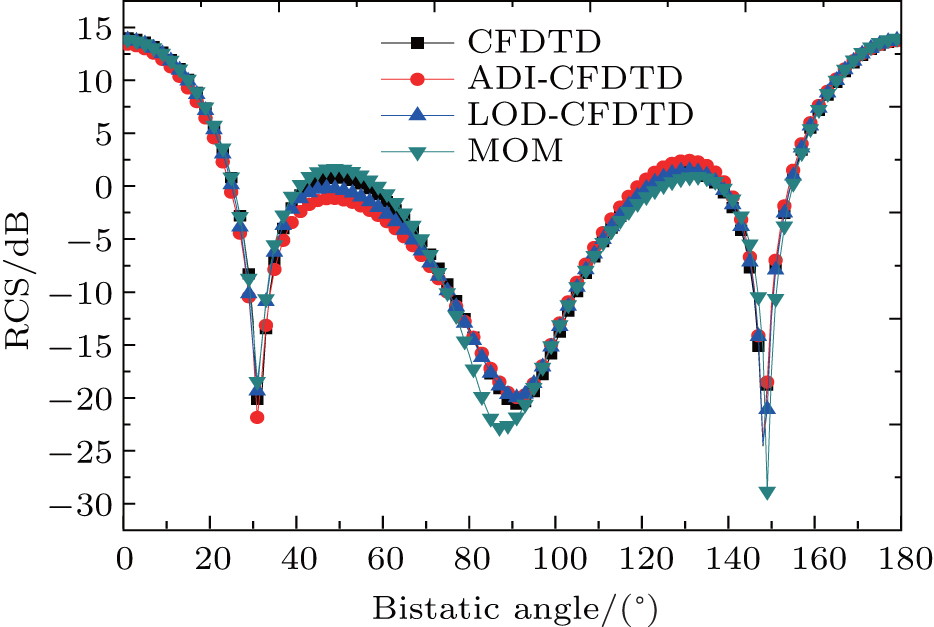 | Fig. 13. Bistatic RCS of two PEC elliptic cylinders obtained from four methods. |
Moreover, a comparison between the CFDTD, ADI-CFDTD and LOD-CFDTD methods in terms of execution time and memory usage for calculating the RCS of this example is shown in Table 2. In Table 2, with the same grid density, the CPU time for LOD-CFDTD is less than that for CFDTD and ADI-FDTD while maintaining the acceptable accuracy.
| Table 2. Comparison of computer resources for the two PEC elliptical cylinders using CFDTD, ADI-CFDTD, and LOD-CFDTD. |
An efficient unconditionally stable LOD-CFDTD method has been proposed for solving 2D scattering problems in this paper. Unlike the staircasing approximation scheme, which often results in the expensive cost of CPU time and memory requirement in LOD-FDTD, the conformal grid is used to model the structures with curved boundaries in the proposed approach, whereas the standard Yee grid is used for the remaining domains. The stability and numerical dispersion of LOD-CFDTD are analytically investigated. It is proved that the LOD-CFDTD method is still unconditionally stable. Moreover, the conformal grids which account for a small percentage of the whole grids have little effect on the numerical dispersion. Two numerical examples of 2D scattering problems illustrate that the proposed method can effectively reduce the CPU time while its results are in good agreement with the conventional CFDTD and ADI-CFDTD methods. In future work, the three-dimensional (3D) LOD-CFDTD will be introduced to solve large and complicated EM problems.
| 1 |
|
| 2 |
|
| 3 |
|
| 4 |
|
| 5 |
|
| 6 |
|
| 7 |
|
| 8 |
|
| 9 |
|
| 10 |
|
| 11 |
|
| 12 |
|
| 13 |
|
| 14 |
|
| 15 |
|
| 16 |
|
| 17 |
|
| 18 |
|
| 19 |
|
| 20 |
|
| 21 |
|
| 22 |
|
| 23 |
|
| 24 |
|
| 25 |
|
| 26 |
|
| 27 |
|
| 28 |
|
| 29 |
|
| 30 |
|
| 31 |
|
| 32 |
|
| 33 |
|
| 34 |
|
| 35 |
|