


Stochastic stability of the derivative unscented Kalman filter
[Hu Gao-Ge†a)  , Gao She-Sheng
a) , Zhong Yong-Minb) , Gao Bing-Binga) ]
, Gao She-Sheng|
|


†Corresponding author. E-mail: hugaoge1111@126.com
*Project supported by the National Natural Science Foundation of China (Grant No. 61174193) and the Doctorate Foundation of Northwestern Polytechnical University, China (Grant No. CX201409).
This is the second of two consecutive papers focusing on the filtering algorithm for a nonlinear stochastic discrete-time system with linear system state equation. The first paper established a derivative unscented Kalman filter (DUKF) to eliminate the redundant computational load of the unscented Kalman filter (UKF) due to the use of unscented transformation (UT) in the prediction process. The present paper studies the error behavior of the DUKF using the boundedness property of stochastic processes. It is proved that the estimation error of the DUKF remains bounded if the system satisfies certain conditions. Furthermore, it is shown that the design of the measurement noise covariance matrix plays an important role in improvement of the algorithm stability. The DUKF can be significantly stabilized by adding small quantities to the measurement noise covariance matrix in the presence of large initial error. Simulation results demonstrate the effectiveness of the proposed technique.
As a relatively new nonlinear filtering algorithm, the unscented Kalman filter (UKF) is an improvement to the extended Kalman filter (EKF).[1, 2] It uses a finite number of sigma points to propagate the probability of state distribution through the nonlinear dynamics of a system, thus reducing linearization errors involved in the EKF. Consequently, the UKF has received great attention in many areas such as control theory, aerospace navigation, eye tracking, and information fusion.[3– 9] However, in the case of nonlinear stochastic systems with linear system state equation, such as the target tracking system[5] and the tightly coupled INS/GPS integrated system, [10] the UKF causes a great amount of redundant computation in the prediction process. This is because the system state equation is linear while it is still used for each of the chosen sigma points in turn to yield a transformed sample to calculate predicted mean and covariance.
To overcome this limitation of the UKF, a derivative unscented Kalman filter (DUKF) was reported in our previous work[1] to reduce the computational complexity by incorporating the concise form of the original Kalman filter (KF) in the prediction process. The DUKF avoids the extra computational load involved in the implementation of the UKF and also inherits the excellent properties of the UKF in dealing with nonlinear filtering problems. However, similar to the UKF, the DUKF is sensitive to the initial error, that is, the DUKF may diverge if the initial state is not sufficiently close to the actual state.
Studies have been dedicated to the stability analysis of the UKF. Based on the new formulation of the first-order linearization technique developed by Boutayeb et al., [11, 12] Xiong et al. proved that, if the process noise covariance matrix is properly chosen, the UKF for a nonlinear system with linear measurements is exponentially bounded in mean-squared estimation error.[13] However, this result is not generic since the nonlinear system considered is a quite simple case in the filed of nonlinear filtering. By taking into account the approximation error of unscented transformation (UT) in the calculation of the cross-correlation covariance matrix between the predicted state and measurement, Xiong et al. extended the result to a general nonlinear stochastic system with nonlinear measurements.[6, 14] However, this study requires a strong coupling relationship between the designed covariance matrices of the process and measurement noises and the sufficient conditions for the designed noise covariance matrices to guarantee the boundedness of estimation error are totally given by a sophisticated construction, thus leading to the difficulty in using the achieved result. Xu et al. also studied the stability analysis of the continuous-time UKF.[15] This study proves that the estimation error will be bounded if the system satisfies a detectability condition and both the initial estimation error and the disturbing noise terms are small enough.[16] However, in the implementation of the UKF, it is difficult to keep the initial estimation error small. Just recently, Li and Xia analyzed the error behavior of the UKF for a nonlinear stochastic system with intermittent measurement.[17] However, this study only provides some indications for the impact of intermittent observations on the stochastic stability of the UKF, without concrete results. To the best of our knowledge, there has been limited research on the analysis of the error dynamics of the DUKF in the presence of large initial error.
This paper focuses on the stochastic stability of the DUKF with poor initial conditions. Based on some standard results about the boundedness of stochastic processes and using the second method of Lyapunov, it is proved that the estimation error of the DUKF remains bounded under certain conditions. Motivated by the assumption that the approximation error of UT in calculating the cross-correlation covariance matrix between the predicted state and measurement is small enough, the coupling relationship between the process noise covariance matrix and designed measurement noise covariance matrix is removed from the sufficient conditions to guarantee the stochastic stability of the DUKF. Furthermore, the impact of the measurement noise covariance matrix on the error behavior is analyzed. It is demonstrated that by adding small quantities to the measurement noise covariance matrix, the stability of the DUKF can be achieved while maintaining certain accuracy. The above results are verified through numerical simulations on three example systems in the presence of large initial error.
Throughout this paper, | | · | | denotes the Euclidian norm of real vectors or the spectral norm of real matrices, E (x) is the expectation value of x, and E (x| y) is the expectation value of x conditional on y.
In order to conduct the stability analysis, let us briefly review the concept of the DUKF at first.
Consider the nonlinear discrete-time system represented by


where xk ∈ Rn and zk ∈ Rm denote the state and measurement vector at time step k, Φ k/k− 1 is the discrete state transition matrix, h(· ) is the nonlinear function describing the measurement model and is assumed to be continuously differentiable, and wk and vk are the uncorrelated zero-mean Gaussian white noise processes with covariances

The DUKF deterministically chooses a set of weighted sigma points to capture the specific information of the predicted mean and covariance rather than the priori ones. In terms of the prediction process, the DUKF has the same form as the KF, thus avoiding the extra computational load of the UKF caused by the UT. In the update process, the predicted measurement, measurement covariance, and cross-correlation covariance are calculated by the statistics of chosen sigma points and transformed sigma points yielded through the nonlinear measurement equation. Thus, the DUKF provides a filtering solution to retain the nonlinearity of the nonlinear measurement equation with at least second-order accuracy.
The procedure for implementing the DUKF can be summarized as follows.[1]
Step 1 Give the state estimate x̂ k− 1 and the error covariance matrix P̂ k− 1.
Step 2 Prediction As the system state equation is linear, the predicted mean and covariance are performed with the same equations as the KF,


Step 3 Sigma points selection A set of weighted sigma points are selected from the predicted mean and covariance of the state. These sigma points are obtained by

where a ∈ R is a tuning parameter denoting the spread of the sigma points around x̂ k/k− 1 and is generally set as a small positive value, and 
Step 4 Update The transformed sigma points yielded through the nonlinear measurement model are

The predicted measurement and the measurement covariance are given by


and the cross-correlation covariance matrix between the predicted state and measurement is expressed as

where

The Kalman gain is determined as

Then, the state x̂ k and the corresponding error covariance matrix Pk can be updated by


Step 5 Repeat Steps 1 to 4 for the next sample.
Define the estimation error and prediction error by


Substituting Eqs. (1) and (4) into Eq. (15) gives

Define the innovation vector as

Expanding zk as a Taylor series about x̂ k/k− 1 yields

where the i-th term in the Taylor series for h(· ) is given by
where xj denotes the j-th component of x.
Expanding ẑ k/k− 1 given by Eq. (8) by a Taylor series yields
Substituting Eqs. (18) and (19) into Eq. (17), the innovation vector z̃ k becomes

where Hk = ∂ h(x)/∂ x| x= x̂ k/k− 1, and Δ (x̃ k/k− 1) denotes the second- and higher-order moments in the Taylor series.
In order to simplify the error expression, the unknown instrumental diagonal matrices α k = diag(α 1, k, α 2, k, … , α m, k) are introduced to model errors due to the first-order linearization, [11, 12] leading to the following exact equality:

The real cross-correlation covariance matrix between the predicted state and measurement is

Similar to Eq. (21), the unknown instrumental matrices 

From the presentation of z̃ k given by Eq. (21), the real measurement covariance matrix can be expressed as
Define

A slight modification is made by adding an extra positive definite matrix Δ Rk to the calculated measurement covariance matrix P̂ ẑ k/k− 1, where the role of Δ Rk to guarantee the stability of the DUKF is shown in Section 3.2. Then the calculated measurement covariance matrix may be written as

where 
Thus, from Eqs. (23) and (25), it is verified that


Substituting Eq. (26) into Eq. (13) and applying the matrix inversion lemma yield

Based on the matrix inversion lemma and Eq. (27), equation (26) can also be rewritten as
In order to analyze the dynamics of the estimation error (14), we introduce the following standard result for the boundedness of stochastic processes.
Lemma 1 Assume that ς k is a stochastic process, and there is a stochastic process Vk (ς k) together with real numbers vmin, vmax > 0, μ > 0, and 0 < λ ≤ 1 such that

and

Then, the stochastic process ς k is exponentially bounded in mean square, i.e.,

This lemma can be found in Ref. [18].
Theorem 1 Consider the nonlinear stochastic systems given by Eqs. (1) and (2) and the modified DUKF described by Eqs. (4)– (8), (10)– (13), and (25). Let the following assumptions hold for every k ≥ 0.
(i) There exist real constants ϕ min, ϕ max, cmin, cmax, hmin, hmax, η max, κ max > 0 such that the following bounds are fulfilled:


where hmin ≤ cmax.
(ii) There exist real constants 


(iii) There exists a real constant ε max > 0 such that the following matrix norm is bounded via:

where 
Proof Define a Lyapunov function

From Eq. (39) it follows that

To satisfy the requirement of Lemma 1, it requires an upper bound on E [Vk (x̃ k) | x̃ k− 1] – Vk− 1 (x̃ k− 1) as given by Eq. (30).
Substituting Eq. (12) into Eq. (14) and using Eqs. (15)– (17) and (21), it can be verified that
Due to the fact that wk and vk are the uncorrelated Gaussian white noise processes and x̃ k− 1 is uncorrelated to wk and vk, substituting Eq. (44) into Eq. (30) and taking the conditional expectation yield

Considering the property of the condition expectation E(x̃ k− 1| x̃ k− 1) = x̃ k− 1, equation (45) can be further expressed as

Substituting Eq. (28) into the first item of Eq. (46) gives
Substituting Eq. (27) into the first item of Eq. (47) yields

From Eqs. (26) and (28), it can be verified that
Then, by substituting Eqs. (48) and (49) into Eq. (47), we obtain

Substituting Eq. (5) into 

Considering Eq. (51), equation (50) can be expressed as


Hence, the following equality is obtained by substituting Eq. (52) into Eq. (46):
Denote

and
Since both sides of Eq. (54) are scalars, taking the trace does not change their values. Substituting Eq. (28) into Eq. (54) and using Tr(AB) = Tr(BA), we have
Apparently, μ k > 0. Using Eqs. (35)– (40), we have

Under assumptions (32) and (37)– (41), it can be verified that
Thus, from Eqs. (32)– (34) and (37)– (40), we can obtain

Obviously, it follows from Eq. (59) that

Consequently, applying Lemma 1 with Eqs. (53), (57), and (59), the inequality

is satisfied. This complements the proof of the boundedness of x̃ k.
Theorem 1 provides the sufficient conditions to guarantee the stochastic stability of the DUKF. It also clearly defines the connection between the design of the measurement noise covariance matrix and the filter stability. To ensure the stability of the DUKF, it requires the matrix 

Remark 1 The condition hmin ≤ cmax can be relaxed as 

Remark 2 The rationality of assumption (41) lies in the fact that the error introduced by the UT for estimating the posterior mean and covariance of the state of any Gaussian and nonlinear system is in at least second-order accuracy.[9, 19]
Remark 3 The assumption (39) will be fulfilled if the matrices Φ k/k− 1 and Hk satisfy the nonlinear uniform observability condition.[20, 21]
Remark 4 Even though the condition (37) in Theorem 1 provides a theoretical criteria to obtain Δ Rk, it is difficult to acquire the analytical solution for the bounds on Δ Rk. This is because the determination of the parameters 

The result described in Section 3 proves that the estimation error of the DUKF will remain bounded if the considered nonlinear system satisfies certain conditions. It shows that the stability of the DUKF can be significantly improved by adding small quantities to the measurement noise covariance matrix. It also excludes the requirement of small initial estimation error.
In this section, simulations have been conducted based on three real-world systems to illustrate the effectiveness of the proposed technique. The performance of the modified DUKF with an extra positive definite matrix Δ Rk is comprehensively evaluated in comparison with the original DUKF.
Consider a radar target tracking system based on two-dimensional Cartesian coordinates.[5] The target moves according to a constant velocity (CV) model, and the radar measures the azimuth angle and slope distance of the target. Denote the state vector as xk = [x1, k, x2, k, x3, k, x4, k]T, where x1, k and x2, k are the displacement and velocity in the x axis, x3, k and x4, k are the corresponding components in the y axis. The system state equation and the measurement equation are described as


The covariance matrices of wk and vk are

The initial conditions for the system and filters are taken as

The initial covariance matrix is chosen as

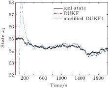
Figure 1 depicts the state x2, k and its estimates x̂ 2, k obtained by the DUKF and the modified DUKF with an extra additive matrix Δ Rk = diag(72, 0.0012) (named the modified DUKF1), respectively. As shown in Fig. 1, in the case of large initial error for x1, k, the DUKF fails to converge with the noise covariance matrices (64). However, as the designed extra positive definite matrix Δ Rk is added to Rk so that the assumption (37) in Theorem 1 is fulfilled, the estimation error of the modified DUKF1 remains bounded for the above initial conditions. This verifies that the stability of the DUKF can be improved by adding small quantities to the measurement noise covariance matrix.
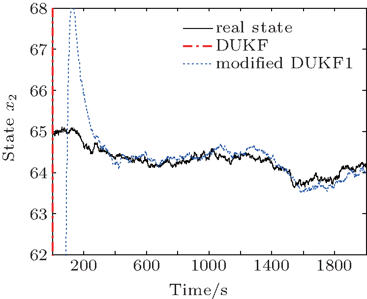 | Fig. 1. State x2, k and its estimates x̂ 2, k for the radar target tracking system. |
Monte Carlo simulations were conducted to analyze the impact of the extra positive definite matrix Δ Rk on the error behavior. In addition to the DUKF and the modified DUKF1 with Δ Rk = diag(72, 0.0012), the modified DUKF with another extra additive matrix Δ Rk = diag(302, 0.0152) (named the modified DUKF2) was also used to estimate the state x2, k. The Monte Carlo simulations were carried out for 10 times, yielding 10 realizations of the state and measurement trajectories. The mean square errors (MSEs) of the three filters were calculated by averaging the square error between x2, k and x̂ 2, k over 10 trials. The results are shown in Fig. 2.
It can be seen from Fig. 2 that the MSE of the DUKF diverges. However, due to the enlargement of the measurement noise covariance matrix, the MSEs of the modified DUKF1 and the modified DUKF2 remain bounded. Figure 2 also shows that the MSE of the modified DUKF2 is much worse than that of the modified DUKF1. It confirms that the larger the extra positive definition matrix Δ Rk is, the larger the estimation error will be. Therefore, it requires the extra positive definition matrix Δ Rk to be chosen properly to balance the stability and accuracy of the modified DUKF.
 | Fig. 2. Mean square errors of the three filters for state x2, k in the radar target tracking system. |
Trials were conducted to evaluate the efficiency of the proposed technique in stabilizing the DUKF with large initial error for a tightly coupled INS/GPS integrated system. The system state equation and measurement equation of the tightly coupled INS/GPS integration for the DUKF are given in Refs. [1] and [22]– [24], respectively. The system state vector is defined as

where (δ vE, δ vN, δ vU) is the velocity error, (ϕ E, ϕ N, ϕ U) the attitude error, (δ L, δ λ , δ h) the position error, (ε x, ε y, ε z) the gyro constant drift, (∇ x, ∇ y, ∇ z) the accelerometer zero-bias, and (bp, bf) the range bias and range drift related to the GPS receiver clock.
The measurement vector is taken as

where δ ρ is the range error which can be obtained by subtracting the estimated ranges of the INS from the pseudorange measurements of the GPS receiver.[1]
The aircraft trajectory, which was designed for a complex high-dynamic aircraft flight in the real world, is shown in Fig. 3. The flight involves various maneuvers such as climbing, pitching, rolling and turning. The simulation parameters are given in Table 1. It can be seen that the initial position error is very poor. The simulation time is 3600 s and the filtering period is 1 s.
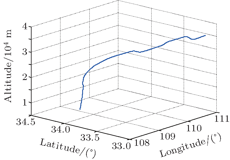 | Fig. 3. Aircraft trajectory. |
| Table 1. Simulation parameters for the tightly coupled INS/GPS integrated system. |
The initial error covariance matrix is taken as
The covariance matrices of the process noise and measurement noise are
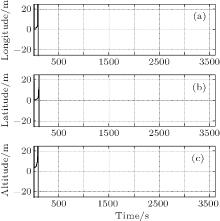
Figures 4 and 5 depict the position errors obtained by the DUKF and the modified DUKF with an extra additive matrix Δ Rk = (20 m)2I4× 4 (named the modified DUKF1). It can be seen that the position errors of the DUKF diverge significantly. This indicates that the DUKF is sensitive to the large initial error and performs in a subpar fashion. However, with the particular design of the modified measurement noise covariance matrix 
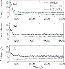
Furthermore, the MSEs of the position errors by the DUKF, the modified DUKF1 and the modified DUKF with another extra additive matrix Δ Rk = (50 m)2I4× 4 (named the modified DUKF2) were computed from 10 times of Monte Carlo simulations. The results are shown in Fig. 6, demonstrating the similar trend to that in Fig. 2. It can be observed that the MSE curve of the DUKF fails to converge, while the modified DUKF1 and DUKF2 remain bounded. Compared with the modified DUKF1, the MSE of the modified DUKF2 is much larger. These plots confirm that with a properly chosen extra positive definition matrix Δ Rk, the modified DUKF is robust. However, setting a very large value for Δ Rk will decrease the MSE accuracy of the modified DUKF.
 | Fig. 4. Position errors ((a) longitude, (b) latitude, (c) altitude) obtained by the DUKF for the tightly coupled INS/GPS integrated system. |
 | Fig. 5. Position errors ((a) longitude, (b) latitude, (c) altitude) obtained by the modified DUKF1 for the tightly coupled INS/GPS integrated system. |
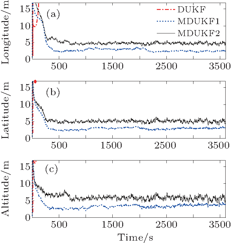 | Fig. 6. MSEs of the position errors ((a) longitude, (b) latitude, (c) altitude) by the DUKF, modified DUKF1 and modified DUKF2 for the tightly coupled INS/GPS integrated system. |
The bearings-only tracking system[25] is also considered to verify the effectiveness of the proposed technique. The bearings-only tracking system is composed of two sensors to track a moving target, where each sensor obtains only an angle measurement related to the system state. The state vector is denoted as xk = [x1, k, x2, k, x3, k, x4, k]T, where the meanings of the components are the same as those in Section 4.1. The target moves according to the CV model described by Eq. (62).
According to the principle of two-position cross-point, the measurement equation can be established as
where d = 5000 m is the distance between the two sensors.
The covariance matrices of wk and vk are selected as

The initial conditions for the system and filters are

The initial covariance matrix is taken as

Figure 7 depicts the state x2, k and its estimates x̂ 2, k by the DUKF and the modified DUKF with an extra additive matrix Δ Rk = diag(0.000052, 0.000052)× π /180 (named the modified DUKF1). Figure 8 illustrates the MSEs of state x2, k by the DUKF, the modified DUKF1, and the modified DUKF with another extra additive matrix Δ Rk = diag(0.00252, 0.00252)× π /180 (named the modified DUKF2) calculated from 10 times of Monte Carlo simulations. The similar phenomena to that in Sections 4.1 and 4.2 can also be observed from these figures. On one hand, in the presence of large initial error for x1, k, the DUKF diverges significantly with the noise covariance matrices (72). However, as the designed extra positive definite matrix Δ Rk = diag(0.000052, 0.000052)× π /180 is added to Rk, the estimation error of the modified DUKF1 remains bounded for the large initial error. On the other hand, with the enlargement of the extra additive matrix from Δ Rk = diag(0.000052, 0.000052)× π /180 to Δ Rk = diag(0.00252, 0.00252)× π /180, the MSEs of the modified DUKF2 become much larger than that of the modified DUKF1. These verify the result described in Section 3 that the stability of the DUKF can be improved by adding small quantities to the measurement noise covariance matrix, while a very large extra additive matrix will decrease the accuracy of the modified DUKF.
 | Fig. 7. State x2, k and its estimates x̂ 2, k for the bearings-only tracking system. |
 | Fig. 8. Mean square errors of the three filters for state x2, k in the bearings-only tracking system. |
The paper studies the error behavior of the DUKF for a nonlinear stochastic discrete-time system with linear system state equation. It proves that the estimation error of the DUKF will remain bounded in mean square if the system satisfies certain conditions. It also clearly defines the connection between the design of the measurement noise covariance matrix and the stochastic stability of the DUKF. The proposed technique shows that, by adding small quantities to the measurement noise covariance matrix, the DUKF can be stabilized without the assumption of small initial estimation error. Theoretical analysis and simulation results demonstrate that, with an enlargement of the measurement noise covariance matrix, the stability of the DUKF can be significantly improved despite large initial error. However, the value of the extra positive definite matrix Δ Rk needs to be chosen properly to balance the stability and accuracy of the modified DUKF.
Future research work will focus on the combination of the proposed technique with artificial intelligence such as advanced expert systems, neural networks, and genetic algorithms to automatically determine the value of Δ Rk for achieving the optimal balance between the stability and accuracy.
| 1 |
|
| 2 |
|
| 3 |
|
| 4 |
|
| 5 |
|
| 6 |
|
| 7 |
|
| 8 |
|
| 9 |
|
| 10 |
|
| 11 |
|
| 12 |
|
| 13 |
|
| 14 |
|
| 15 |
|
| 16 |
|
| 17 |
|
| 18 |
|
| 19 |
|
| 20 |
|
| 21 |
|
| 22 |
|
| 23 |
|
| 24 |
|
| 25 |
|