


Possible magnetic structures of EuZrO3*
[Hu Ai-Yuan† , Qin Guo-Ping, Wu Zhi-Min, Cui Yu-Ting]
, Qin Guo-Ping, Wu Zhi-Min, Cui Yu-Ting]
|
|


†Corresponding author. E-mail: huaiyuanhuyuanai@126.com
*Project supported by the National Natural Science Foundation of China (Grant Nos. 11404046, 11347217, and 61201119), the Basic Research Foundation of Chongqing Education Committee, China (Grant No. KJ130615), and the Chongqing Science & Technology Committee, China (Grant Nos. cstc2014jcyjA50013 and cstc2013jjB50001).
A comprehensive research of the antiferromagnetic (AFM) structures of perovskite-type EuZrO3 is carried out by use of the double-time Green’s function. Two possible types of AFM configurations are considered, and theoretical results are compared with experimental results to extract the values of parameters J1, J2, and D. The obtained exchanges are employed to calculate the magnetic susceptibility, which is then in turn compared with the experimental one. Therefore, we think that the magnetic structure of EuZrO3 may be an isotropic G-type structure or an anisotropic A-type structure.
Multiferroics with magnetoelectric properties have recently become the focus of intensive research due to the coexistence of both magnetic and electric ordering parameters, which is of interest for novel exciting applications like magnetic field sensors, tunable microwave devices, multiple state memory elements, and spintronic devices.[1– 5] For their practical applications, detailed knowledge about their crystal structures and magnetic structures is necessary.
Among the most studied multiferroics, the perovskite oxide (ABO3) has a prototype cubic structure. The EuZrO3 may be a typical crystal. Its crystal structure is quite similar to EuTiO3, [6, 7] i.e., isotropic G-type antiferromagnet (AFM). A previous study showed that EuZrO3 was a cubic (space group Pm
As for the aspect of magnetic structure, experimental results indicated that EuZrO3 behaved as an AFM character below about 4.1 K.[6, 9, 10] Its magnetic crystal structure was also very similar to EuTiO3. General investigations conjectured that its magnetic crystal structure was a G-type AFM, [6, 9, 11] although there had been no further experimental evidence. Nevertheless, for ABO3-type AFM perovskite oxides where magnetic ions are located on a simple cubic lattice, there may exist three types of AFM orderings, namely, G-, A-, and C-types, as shown in Fig. 1. Thus some efforts have been devoted to understanding its magnetic structures.[9, 11– 13]
Alho et al. studied the magnetic properties of EuZrO3 based on an isotropic G-type AFM by use of the mean field theory (MFT) and Monte Carlo simulation.[13] The results agreed with experimental data in a high temperature range, but deviated from experimental results at T ≤ TN. Based on the MFT, Zong et al.[9] analyzed three possible magnetic structures for EuZrO3, i.e., G-, A-, and C-types. The C-type AFM structure was ruled out. Therefore, the magnetic structure of EuZrO3 may be an isotropic G- or A-type AMF.[9] However, they compared EuZrO3 with a series of similar magnetic structures containing Eu2+ perovskite oxides, and thought that the magnetic structure of EuZrO3 was an isotropic G-type AMF, while the isotropic A-type AMF could not be ruled out. Meanwhile, they also pointed out that the spin canting may exist in EuZrO3 since Eu2+ is an S-state ion. It showed that the magnetic structure of EuZrO3 may have an anisotropy. Since the single-ion anisotropy or dipole– dipole interactions may lead to spin canting.[9]
 | Fig. 1. Schematic depiction of the G-, A-, and C-type antiferromagnetic structures. The arrow refers to spin orientation. |
In our previous investigation, we did a comprehensive discussion about three possible perovskite-type magnetic structures (i.e., isotropic G-, A-, and C-type AFM) in EuZrO3 based on the many-body Green' s function method (GFM) and MFT.[13] Our results indicated that the isotropic A- and C-types AFMs were ruled out. The susceptibility of isotropic G-type AFM agreed with the experimental one below and near critical temperature, but deviated from experimental results in a high temperature range. The difference between theoretical and experimental results may be due to there being no consideration of anisotropy. However, the G- and A-type AFMs with a single-ion anisotropy have not been discussed. In this paper, we intend to consider anisotropic G- and A-type AFMs to discuss the possible magnetic structure of EuZrO3 by means of GFM. The rest of this paper is organized as follows. In Section 2, the formulas are given that relate the parameters to the crtical temperature, Curie– Weiss temperature, and susceptibility. In Section 3, the numerical results and discussion are presented. In the last section, we draw some conclusions from the present study.
The effect of single-ion anisotropy or dipole– dipole interactions on the magnetic property of the system has been discussed comprehensively in a previous investigation.[14] Generally, the strength of dipole– dipole interaction is very weak compared with the single-ion anisotropy.[15] It is usually neglected if the single-ion anisotropy is considered. Thus our Hamiltonian will only include a single-ion anisotropy. The dipole– dipole anisotropy will not be considered here. In the following, the G- and A-type AFM Hamiltonian with the single-ion anisotropy will be studied. The G- and A-types of the AFM structures are depicted in Fig. 1, and their Hamiltonian can be written as
Here, Jij and Jnm are the nearest-neighbor (nn) and second-nearest-neighbor (nnn) exchange parameters, respectively; the sums 〈 i, j〉 and [i, j] run over the nn and nnn lattice sites, respectively; D is the single-ion anisotropy parameter, and D ≥ 0. The last term in Eq. (1) is Zeeman energy when an external field h along the z axis is exerted. For each type, the AFM lattice can be partitioned into two sublattices, denoted by a and b, respectively, although the partition may be different for different types. It is assumed that the sublattice magnetizations are along the z direction. The spin averages of the two sublattices are hereafter denoted as 
Some more words should be added to exchange parameters Jij and Jnm. In the G-type magnetic structure, all the nn spins are antiparallel to each other, and all the nnn spins are parallel to each other. Therefore, in Eq. (1), we simply put down Jij = J1 and Jnm = J2, where in this convention J1 < 0 and J2 > 0. In the A-type magnetic structure, each site spin has some parallel and antiparallel nn and nnn spins. For this case, in Eq. (1), Jij = − J1 (J1) for parallel (antiparallel) nn spins, and Jnm = J2 (− J2) for parallel (antiparallel) nnn spins.
We obtain the formulas for calculating the magnetization and zero-field susceptibility of G- and A-type AFMs by the GFM.[16] The derivation is lengthy for G- and A-type AFMs based on the standard routine of GFM. As an example, we only intend to give the derivation details of A-type AFM here. For G-type AFM, the corresponding physical quantity can also be derived by a similar procedure. Meanwhile, in order to conveniently give the expressions of the critical temperature and zero-field susceptibility of G- and A-type AFMs, a subscript G or A is attached to TN and χ to denote which type of structure the quantities belong to.
Following the standard routine of GFM, the Green’ s function is defined as follows:

where H = a, b, and uH is the Callen parameter.[16] Then the equation of the motion of the Green’ s function will be obtained by standard procedure.[16] In this course, the higher-order Green functions need to be decoupled. For the terms concerning exchange interaction in Eq. (1), we use random phase approximation (RPA) decoupling:[16]

For the terms concerning the single-ion anisotropy, we adopt the Anderson– Callen’ s decoupling (CAD):[16]

where

Define

where N is the number of lattice sites, and the summation of wave vector k runs over the first Brillouim zone. For uH = 0, we have θ (uH) = 2mH. The Green’ s function converts Fourier-transform into wave vector space. After that, the equal-time correlation function 
 |
where H = a, b, and kB is the Boltzmann constant.


By the relation

the magnetization is expressed by the following formula:[16]

In this section, we use our solutions of the Green’ s functions to derive the formulae for the critical temperature and susceptibility in the paramagnetic phase.
First of all, we estimate the critical temperature TAN which is obtained from the limiting of Eq. (17). For h = 0, we obtain ma = − mb. As the temperature approaches to the critical point, the magnetization ma approaches to zero. The equation

is found. This leads to

Inserting Eqs. (10) and (11) into the above equation for h = 0 and ma = − mb, we obtain the critical temperature
where

Secondly, when h → 0 and T → TAN, the sublattice magnetization mH is a small quantity. Therefore, the zero-field sublattice susceptibility can be written as χ H = mH/h. Thus, at T → TAN, by Eqs. (9)– (11) and (17), we obtain

At the critical point, the zero-field susceptibility reaches its maximum. Based on Eqs. (5), (9)– (15), and (22), the susceptibility maximum can be obtained as
It should be pointed out that the sublattice magnetization has a linear relation with the external field (i.e., ma, b = ± m0+ χ h) at h → 0, where m0 is spontaneous magnetization. At T > TN, the spontaneous magnetization is zero, and two zero-field sublattice susceptibilities are equal, i.e., χ a = χ b. According to Eq. (23), the zero-field susceptibility of the system can be expressed as χ = χ a = χ b. Similarly, the relation of Eq. (22) is also satisfied for T > TAN. Combining Eqs. (5) and (9)– (15) with Eq. (22), after a tedious calculation, the zero-field sublattice susceptibility is given by

to the third order of T, where F is the Curie constant; Θ A is the Curie– Weiss temperature, which is given by>

By a procedure similar to the above procedure, the TGN, χ (TGN), and Θ G of G-type AFM can also be obtained. We do not intend to give its details here. However, the final formulas are presented as follows:


where

By Eqs. (23) and (27), it is seen that the susceptibility maxima of A- and G-type AFMs are independent of D, and the susceptibility maxima of G-type AFM solely depend on the nn exchange parameter J1. By means of the formulas derived from the GFM, we are able to determine J1, J2, and D in terms of the experimentally measured TN, χ (TN), and Θ . The measured values of TN, χ (TN), and Θ of the material are listed in Table 1.
| Table 1. Experimental values of TN, χ (TN), and Θ of EuZrO3. |
We derive the expressions of the critical point TGN, the susceptibility maximum χ (TGN), and the Curie– Weiss temperature Θ G, i.e., Eqs. (26), (27), and (28) which are expressed by the three parameters J1, J2, and D. It can be seen that the maximum susceptibility of the G-type structure is only related to the nn exchange parameter J1, but not to J2 and D. This feature helps us to easily determine J1 of the G-type structure without influencing J2 and D. After J1 is calculated by Eq. (27), the other parameters J2 and D are evaluated by Eqs. (26) and (28). Firstly, inserting the J1 and experimental Θ G[6] values into Eq. (28) (note that S = 7/2[6, 9]), the relation between J2 and D is obtained, i.e., J2 = 0.0136172 − 0.047619D. When J2 = 0, it is reckoned that D = 0.286. We fix J2 > 0 and D ≥ 0. Hence, the D value is confined in a range 0 ≤ D < 0.286. If D is presumed to be a value, the value of J2 is obtained by J2 = 0.0136172 − 0.047619D. Then the J1, J2, and D values are put into Eq. (26) to yield TGN to see whether it agrees with the experimental result. Note that the χ (TGN) and Θ G values are always equal to 1.62462 and 0.1 K based on experimental measurements.[4]
Following this procedure, the relation among TGN, J2, and D is plotted in Fig. 2. Unfortunately, in this way the experimental TGN value fails to be retrieved. In fact, we have tried various possible J1, J2, and D values under the confinement 0 ≤ D < 0.286. The maximum TGN value is always below 3.2 K, less than experimental value 4.1 K, [6] see Fig. 2. One probable reason is that in fitting the experimental data, the Curie– Weiss law is utilized, which merely reflect the information at high temperature. Therefore, the parameters derived from this law are difficult to apply to the temperature region below the critical point.
 | Fig. 2. Critical temperature TGN of the G-type magnetic structure for EuZrO3 determined by Eqs. (27) and (28). Various J2 and D values are tested. Empty circles: J2 varies linearly with D. Empty triangles: J2 = 0. In these two cases, 0 ≤ D < 0.286 K. Empty squares: D = 0. In all the cases, the maximum TGN is 3.19 K, less than the experimental value 4.1 K.[6] |
The experimental results from which we want to deduce the parameters should reflect information about both above and below the critical point. We believe that the measured values at the critical point could do the work, while the Curie– Weiss merely reflects information about above the TN. The two typical quantities at the critical point are TN itself and susceptibility maximum χ (TN).
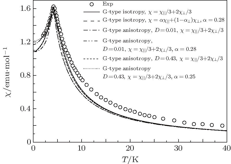 | Fig. 3. Temperature dependences of magnetic susceptibility at h = 0.005 T for G-type AFM. The empty circles represent the experimental data.[6] The solid and dash curves represent isotropic results.[13] The anisotropic results are from this paper. |
We perform the numerical calculation by following two loops. The first loop is that the D value increases from 0 to 1. The second loop is that the J2 starts from 0 to 0.03 (the range of J2 is obtained based on our previous discussion[13]). Finally, the J1, J2, and D values are inserted into Eq. (26) to calculate the TGN value by iterative solution, seeing whether TGN agrees with experimental data. If it agrees with experimental results, a set of possible values of J1, J2, and D will be determined.
Our calculation shows that the maximum value of D is less than 0.44 at J2 > 0. The J2 decreases with the value of D increasing. In order to verify the correctness of our calculated J1, J2, and D values, susceptibility is computed in the whole temperature range, which will be compared with experimental data. The susceptibility χ of a polycrystalline antiferromagnetic system follows the relation[11, 17] that it is one third of parallel susceptibility χ ‖ plus two thirds of perpendicular susceptibility 
It should be pointed out that the isotropic results are always better than the anisotropic results. Our calculations show that the sharp susceptibility will become narrow when the value of D increases. Meanwhile, the corresponding results will also deviate more and more from experimental results. This means that the better results cannot be obtained by turning D. It shows that the anisotropic G-type AFM cannot better retrieve the experimental results. The conclusion is that the anisotropic G-type AFM structure for EuZrO3 is ruled out.
In our previous investigation, the isotropic A-type AFM structure has been ruled out.[13] However, the anisotropic A-type AFM structure has not been discussed. Thus the magnetic structure of the EuZrO3 has not been quite certain, and we here calculate the assumed anisotropic A-type AFM structure to see whether it is possible.
Like the case of G-type AFM, the critical point TAN, the susceptibility maximum χ (TAN), and the Curie– Weiss temperature Θ A of A-type AFM can also be expressed by the three parameters J1, J2, and D, i.e., Eqs. (20), (23), and (25). It is seen that the χ (TAN) is associated with the nn J1 and nnn J2 exchange parameters, and is independent of D, see Eq. (23). Therefore, the range of the J2 value is estimated. We have fixed J2 > 0. In Eq. (23), 4J2 − J1 > 0 should be held, since χ A(TAN) > 0. When J1 = 0, it is reckoned that J2 = 0.0192 K. Hence, the J2 value is confined in the range 0 < J2 < 0.0192 K.
 | Fig. 4. Critical temperature TAN of the anisotropic A-type magnetic structure for EuZrO3 determined by Eq. (20). Various values of J2 and D are tested. Empty circles: J2 varies linearly with D. Empty squares: D = 0. In these two cases, 0 < J2 < 0.0192 K. In Eq. (23), 4J2 − J1 > 0 should be held, since χ A(TAN) > 0. When J1 = 0, it is reckoned that J2 = 0.0192 K. We have fixed J2 > 0. Hence, the J2 value is confined in the range 0 < J2 < 0.0192 K. Empty triangles: J2 = 0. In all the cases, the maximum TAN is 3.13 K, which is less than the experimental value 4.1 K.[6] |
In Fig. 4, the relations among TGN, J2, and D are plotted. It can be seen that the maximum TAN values are always below 3.13 K, less than experimental value 4.1 K.[6] The Curie– Weiss law is valid merely in the high temperature region as has been mentioned. The Curie– Weiss temperature Θ A cannot be utilized to determine these three parameters, similar to the case of G-type AFM.
Therefore, these parameters must utilize the critical temperature TAN and susceptibility maximum χ (TAN) to be determined. Following the computing procedure of G-type AFM, a set of possible values of J1, J2, and D are obtained. Fitting experimental data, the values of J1, J2, and D are determined based on the best fitting result, i.e., J1 = − 0.0769 K, J2 = 10− 5 K, and D = 0.06, see Fig. 5. For comparison, the results of isotropy G- and A-type AFMs are also plotted in Fig. 5. It is seen that the results of isotropic A-type AFM badly deviate from experimental curve. However, the result is improved rapidly when an anisotropy is considered. It agrees with the results of isotropic G-type AFM and the experimental results at below and near the critical point. Similarly, the results can be improved by χ = α χ ‖ + (1 − α )χ ⊥ at T ≤ TN. When α = 0.28, the results of anisotropic A-type AFM agree with experimental data.
Based on the discussion above, two conclusions are obtained. One is that if A-type AFM is a possible magnetic structure of EuZrO3, it is anisotropic. Another is that the magnetic structure of EuZrO3 may be an isotropic G-type AFM or an anisotropic A-type AFM structure since their results are almost identical.
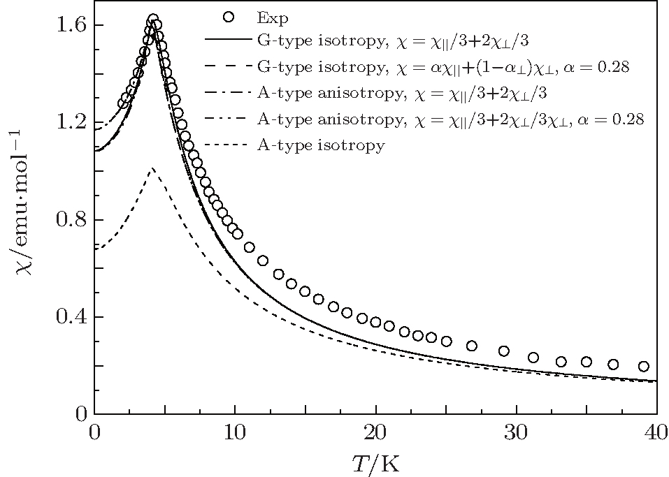 | Fig. 5. Temperature dependences of magnetic susceptibility at h = 0.005 T and D = 0.06 for anisotropic A-type AFM. The empty circles represent the experimental data.[6] The anisotropic A-type AFM results are from this paper. The isotropic G- and A-type AFM results are cited from Ref. [13]. They are reproduced here just for reference. |
 | Fig. 6. Curves of susceptibility versus temperature for (a) isotropic G-type AFM and (b) anisotropic A-type AFM under three magnetic fields h = 0.001 T, 0.005 T, and 0.01 T for D = 0.06. In each panel, the three lines are almost identical. |
Finally, it should be pointed out that equations (23) and (27) are obtained in the zero-field limit. However, the magnetic susceptibility in a weak magnetic field is measured experimentally. Therefore, the influence of a weak magnetic field on the susceptibility should be clarified. Figure 6 shows the curves of susceptibility versus temperature for EuZrO3 at three magnetic fields. The curves for the three fields are almost identical, indicating that the weak magnetic field hardly affects the susceptibility. It is concluded that expressions (23) and (27) as a zero-field limit have no significant difference for the weak field cases. Therefore, using Eqs. (23) and (27) to determine the values of exchange parameters is quite reasonable.
In this paper, we discussed the magnetic structures of the EuZrO3 crystals through a comprehensive study. The GFM is employed. By deriving the formulas of the transition temperature, susceptibility, and Curie– Weiss temperature in terms of the exchange parameters and anisotropy parameter, we are able to determine the parameters by the experimental data. A remarkable feature is that the magnetic susceptibility maxima of the G- and A-type AFMs are associated only with exchange parameters, and are independent of D, and the susceptibility maximum of G-type AFM is decided solely by the nn exchange parameter J1. Our results show that anisotropic G-type AFM is ruled out. The results of isotropic G-type AFM and anisotropic A-type AFM are almost the same, while their susceptibility values deviate from experimental results in the high temperature range. It shows that the isotropic G-type AFM or anisotropic A-type AFM structure is a possible magnetic structure of EuZrO3. Therefore, further experimental and theoretical studies are required to clarify the magnetic structure in EuZrO3.
| 1 |
|
| 2 |
|
| 3 |
|
| 4 |
|
| 5 |
|
| 6 |
|
| 7 |
|
| 8 |
|
| 9 |
|
| 10 |
|
| 11 |
|
| 12 |
|
| 13 |
|
| 14 |
|
| 15 |
|
| 16 |
|
| 17 |
|