
Properties of sound attenuation around a two-dimensional underwater vehicle with a large cavitation number*
[Ye Peng-Cheng† , Pan Guang‡]
, Pan Guang‡]
|
|


†Corresponding author. E-mail: ypc2008300718@163.com
‡Corresponding author. E-mail: panguang601@163.com
*Project supported by the National Natural Science Foundation of China (Grant Nos. 51279165 and 51479170) and the National Defense Basic Scientific Research Program of China (Grant No. B2720133014).
Due to the high speed of underwater vehicles, cavitation is generated inevitably along with the sound attenuation when the sound signal traverses through the cavity region around the underwater vehicle. The linear wave propagation is studied to obtain the influence of bubbly liquid on the acoustic wave propagation in the cavity region. The sound attenuation coefficient and the sound speed formula of the bubbly liquid are presented. Based on the sound attenuation coefficients with various vapor volume fractions, the attenuation of sound intensity is calculated under large cavitation number conditions. The result shows that the sound intensity attenuation is fairly small in a certain condition. Consequently, the intensity attenuation can be neglected in engineering.
Cavitation is the formation of vapor cavities in a liquid, i.e., small liquid-free zones (“ bubbles” or “ voids” ) that are the consequence of forces acting on the liquid. It usually occurs when a liquid is subjected to rapid changes of pressure that cause the formation of cavities where the pressure is relatively low. The performance of equipment in vehicles, especially acoustic detection equipment will be influenced when a high-speed underwater vehicle is encapsulated in a large number of bubbles within a cavity.
A large number of studies on cavitation have been conducted over the past few decades. In recent years, due to the development of computational fluid dynamics (CFD) and computing resources, the numerical studies of mathematical modeling of cavitation have advanced rapidly. For example, the two-phase mixture flow model deals with two-phase continuity equations by employing a volume fraction transport equation.[1– 4] Transport equations have been implemented by many different researchers and have shown reasonable results compared with existing experimental data.[3, 4] The natural cavitating flow around a two-dimensional (2D) symmetrical wedge in shallow water was simulated to analyze the influences of the free surface and the rigid bottom on the cavity based on a single phase mixture model.[5] The Reynolds-averaged Navier– Stokes (RANS) approach showed promising results in the prediction of unsteady cavitation phenomena.[6] Saranjam investigated an underwater high-speed moving body along with cavitation experimentally and numerically.[7] Besides general cavitating flows, many studies on super-cavitating flows have been performed by using experimental and numerical methods. Lindau et al.[8] simulated super-cavitating flow around a flat disk cavitator using the RANS approach. Computational analysis of the turbulent super-cavitating flow around a 2D wedge-shaped cavitator was conducted by Park.[9] Chahine[10] has studied the bubble flow interactions under various conditions and for several families of engineering applications. The results reported in the abovementioned papers demonstrate that the numerical method can be one of the most powerful and beneficial tools for predicting the cavitation of underwater vehicles.
In the classic papers of Foldy and Carstensen, [11] the wave propagation in a bubbly mixture was treated as a problem of multiple scattering by randomly distributed isotropic scatterers representing the spherical bubbles, and the dispersion relation for the mixture was derived. An alternative approach is to treat the mixture as a single phase medium. Wijngaarden[12] defined volume averaged quantities in order to remove the local fluctuations due to scattering and derived the averaged equations based on heuristic, physical reasoning. Commander[13] developed the theory further, in which linear pressure waves in bubbly liquids were discussed. Wang et al., [14] and Wang and Lin[15] obtained the sound attenuation coefficient and the sound speed formulas of the bubbly liquid through solving approximately the linearized equation of wave propagation of bubbly liquids and the dynamic equation of bubbles. Leroy et al.[16] have measured the phase velocity and the attenuation in a monodisperse bubbly medium in a large range of frequencies including the resonance frequency of the bubbles. A model dealing with realistic simulations of the coupled evolution of the cavitation field and the acoustic field has been proposed by Louisnard.[17] Yano et al.[18] studied nonlinear wave propagation in a bubbly liquid. However, in the aforementioned literature the influence of sound intensity attenuation on the underwater vehicles was not studied.
The present study focuses on the sound intensity attenuation resulting from traversing across a cavity around a hemispherical head-form body with a large cavitation number. The numerical simulation based on the viscous multiphase flow model is carried out to study the cavitation flow around a 2D underwater vehicle with a large cavitation number. Based on the formulas of sound attenuation coefficients with various vapor volume fractions, the attenuation of sound intensity is calculated by combining with the vapor volume fraction distributions.
The equations for the mass and momentum conservation are solved to obtain the velocity and pressure fields. The equation for the conservation of mass, or continuity equation, can be written as

where ui is the velocity vector; i indicates the Cartesian coordinates which can be 1 or 2 or 3 and in this paper, i = 2; ρ is the density; t is the time; and m is the subscript indicating the mixture phase.
The equation for the conservation of momentum can be written as

where p is the static pressure, j is the same as i, and the turbulent stress tensor 
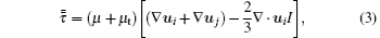
where μ is the viscosity, and the subscript t denotes the turbulence, I is the unit tensor and the second term on the right-hand side is the effect of volume dilation.
The volume fractions of gas, vapor, and liquid phases, denoted as ag, av, al, respectively, are introduced to obtain a set of governing equations describing the multiphase flow of gas, vapor, and liquid phases.
The gas phase should keep continuous

The vapor phase should also satisfy continuity in the phase-transition process

A compatible equation holds for the three phases

Additionally, two individual transportation equations are employed to describe the phase-transition process given in Eq. (5) between the vapor phase and the liquid phase. ṁ + is the mass transfer rate from vapor to liquid

and ṁ − is the mass transfer rate from liquid to vapor
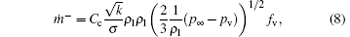
where the values of empirical constants Ce and Cc, which regulate the rates of evaporation and condensation of phases respectively, are 0.02 and 0.01 in Singhal’ s model, [3]pv is the saturation vapor pressure, fv and fg are the mass fractions of vapor and gas, respectively, and σ is the surface tension, which equals 0.07275 N/m.
The density and viscosity of the mixture are calculated as the weighted average of the volume fraction of each phase


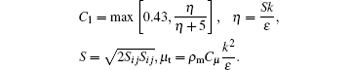
Realizable k– ε is used as the turbulence model, which is based on the Boussinesq hypothesis and the eddy viscosity definition. The transport equation for the turbulence kinetic energy k and dissipation rate ε are obtained from the transport equations, which are

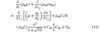
where
In the above equations, Gk represents the generation of turbulence kinetic energy due to the mean velocity gradients, Gb is the generation of turbulence kinetic energy due to buoyancy, YM represents the contribution of the fluctuating dilatation in compressible turbulence to the overall dissipation rate, C2 and C1ε are constants, σ k and σ ε are the turbulent Prandtl numbers for k and ε , respectively. The model constants are C2 = 1.9, C1ε = 1.44, σ k = 1.0, and σ ε = 1.2. Owing to the length limitation of this article, more information is not given but can be found in Ref. [19].
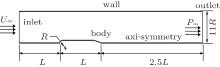
The axisymmetric vehicle has the following geometrical parameters: a head diameter D of 534.4 mm, and a body length L of 7000 mm. Figure 1 shows the computational domain and boundary conditions. The Dirichlet boundary condition, i.e., the specified value of the velocity, is imposed on the inlet boundary. On the exit boundary, the reference pressure with extrapolated velocity and volume fraction value is used. The reference pressure is fixed on the outlet boundary with a desired cavitation number. The axisymmetric condition is imposed on the bottom boundary. A no-slip condition is imposed on the body surface and the upper boundary. The computational domain extends to − L ≤ x ≤ 3.5L and 0 ≤ y ≤ 5.5D in the streamwise and vertical directions, respectively. The domain is set to be large enough to minimize the influence of the inlet boundary.
 | Fig. 1. Boundary condition and domain extent. |
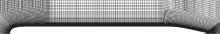
For ensuring the computation accuracy, sufficient structural meshes are needed. Figure 2 shows the mesh near the body. Since the interaction between the near-wall flow and cavity should be taken into consideration, the mesh near the wall of the body is well refined so as to ensure the accuracy of the simulation. The nondimensional normal distance from the wall, i.e., y+ at the wall surface of body is in a reasonable range around 30. In the total domain, structural grids having the node number of 36336 are formed.
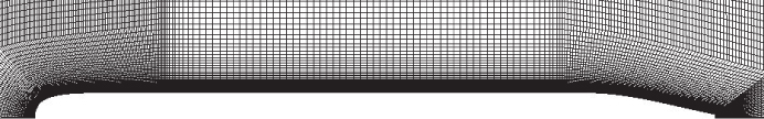 | Fig. 2. Structural grids generated near the body. |
The 2D turbulent cavitating flow in the domain is calculated under the natural cavitation condition. The realizable k– ε turbulence model is used. For convenience, the solver of a commercial CFD software Fluent coupled with the proposed cavitation model[3] are adopted for the calculation.
The continuity equation of the model is given as

where ρ and c are the density and speed of sound of the host liquid respectively, and β is the local fraction of volume occupied by the gas (containing gas and vapor in the paper) given by

where R is the instantaneous radius of the bubbles and n is their number per unit volume. As will be shown, n must be kept constant in taking the time derivative indicated in Eq. (13). This equation is written for the case in which all the bubbles have the same equilibrium radius. Its extension to different bubble sizes is straightforward and is considered later. The bubbly medium is to be described in the average sense and p and u refer to the average pressure and velocity respectively. Although ensemble averaging is conceptually the most satisfactory way to define these quantities, volume averaging may present a simple visualization.
The momentum equation of the model can be written as

Caflisch et al.[20] rigorously proved that the effects due to the relative motion between bubbles and liquid disappear according to the order of the approximations introduced in the model. The velocity field uB of the bubbles can be neglected. Therefore, at this point, only an equation for R is needed to obtain a closed equation set. This equation will be given in the next section. It should be noticed that the radius R must be considered as a field variable R(x, t), where the first argument denotes the position of the bubble.
For a mixture containing bubbles of different sizes, we can define

as the number of bubbles per unit volume with equilibrium radius between a and a + da located in the neighborhood of the point x. Then, the volume fraction β is given, in place of Eq. (14), by

where R(x, a, t) denotes the radius at time t of a bubble located at the position x and having an equilibrium radius a. It should be noted that no time dependence is indicated for the distribution function since the same argument given above to neglect dn/dt shows that f can be considered to be constant during the propagation of the waves. With this expression for β the continuity equation (13) still holds. The momentum equation (15) is also unchanged.
For the case of radial motion of a bubble, an equation accounting approximately for the liquid compressibility is given by Keller in the form of
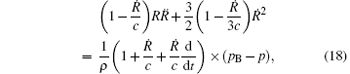
where pB is the liquid pressure at the bubble interface related to the internal pressure p by

with σ and μ denoting the surface tension and the liquid viscosity respectively. For an isolated bubble, the term p in Eq. (18) is defined as the pressure at the position occupied by the bubble if the bubble is absent. In a dilute mixture, to the lowest order in β this quantity coincides with the average pressure defined in the previous section. In this limit, the bubbles do not interact with each other' s field, but with the average field.[12]
The dots in Eqs. (18) and (19) denote total time derivatives that, for a bubble in a mixture, must be interpreted as convective derivatives. However, the same argument given earlier justifies their interpretation as partial time derivatives. We continue to use the dots for simplicity of notation.
To complete the formulation, an equation for the internal pressure p is needed. We start from the enthalpy equation in the gas that, using the equation of state of perfect gases, may be described by

where γ is the ratio of specific heats, K the thermal conductivity, T the temperature, and υ the velocity. If the bubble boundary moves with a velocity much smaller than the speed of sound in the gas, the pressure can be taken to be uniform and the convective derivative with respect to the gas velocity Dp/Dt approximately equates ṗ . With these approximations, equation (20) can be integrated to find an explicit expression for the radial component of the gas velocity as follows:

By imposing the kinematic boundary condition υ = Ṙ at r = R, the above relation becomes an equation for the pressure

With these results, the temperature field can be obtained from the standard form of the energy equation

in which Cp is the specific heat at constant pressure and υ is given by Eq. (21). It may be noted that the equations for u, p, and β , given in the previous section, together with those for the radial motion just presented, constitute a mathematical model valid for a small-amplitude pressure wave. The mixture equations appear to be linearized because, when only a few bubbles are present, even large fluctuations of the bubble volumes can only induce modest average liquid velocities.
Upon elimination of u between Eqs. (13) and (15), with the usual acoustic approximation (i.e., keeping ρ and c constant), we find

The time derivative of β , given by Eq. (17), is

or, in the linear approximation,

and, similarly,

so that

It can be shown that in the linear case, the connection between R and p established by the model is a convolution. This reduces to a simple proportionality only in the case of sinusoidal motion, to which we therefore restrict the analysis from now on. Assuming

and substituting them into the linearized forms of Eqs. (22) and (23), and assuming a proportionality to exp(iω t) and X to be the relative variation of the radius of the bubble, one readily finds that

where

and Df is the gas thermal diffusivity. Note that the function Φ is complex. The quantity p0 in Eq. (29) is the static pressure in the bubble and given by

where p∞ is the equilibrium pressure in the liquid. With the further definition

the linearized form of the Keller equation (18) becomes
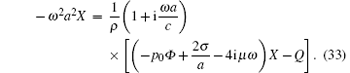
The derivation of Eq. (18) given in Ref. [12] shows that, as an approximation to the equation for a compressible liquid, equation (18) has an error of order c− 2. On the basis of this remark, it is expedient to multiply Eq. (33) by (1 − iω a/c) and to neglect terms of order c− 2. The final result is

where the following definitions


have been introduced to render explicit the similarity of the bubble response to that of a linear oscillator having a natural frequency ω 0 and a damping constant b. However, the dependences of these quantities on the frequency ω of the pressure wave renders this similarity somewhat superficial. The three terms contributing to the damping constant arise from viscous, thermal, and acoustic effects, respectively. The thermal contribution is normally dominant, and it exhibits a strong dependence on ω , particularly near the true resonance frequency.
Substituting Eq. (34) into Eq. (28), we obtain

where the wavenumber in the mixture km is given by the dispersion relation
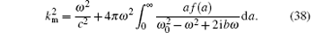
The complex sound speed in the mixture is given by cm = ω m/km and therefore,

Setting

we note that

which shows the phase velocity V of the sound wave to be given by

and the attenuation coefficient A in dB per unit length by

For a monodisperse bubble population with equal equilibrium radius ā , we have

where n is the bubble number per unit volume, and equation (39) becomes

At frequencies well below the natural frequency, equation (45) reduces to

For ω ≪ ω 0, i.e., ω a ≪ c, it may be shown that


With these results, and neglecting for simplicity the surface tension effect, we find


In particular, for values of β that are not too low, equation (49) reduces to the well-known result

For the validation of the numerical method, computational results are compared with the experimental data in the prior literature. It is confirmed that the solution domain, mesh, and boundary conditions are appropriately set up for the given computational conditions with the selected cavitation model of Singhal, et al.[3] and the realizable k– ε turbulence model.
In order to specify the cavitation condition of the flow, a natural cavitation number, σ v, is defined as

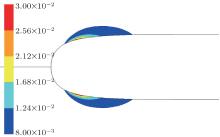
In our computation, the Reynolds number Re is 1.63 × 10⁷ based on the free-stream velocity υ ∞ , which is 60 kN, and the maximum diameter of the vehicle. The cavitation number equals 0.31. The vapor volume fraction around the head of the underwater vehicle is displayed in Fig. 3, where the closured regions denote the cavities, meanwhile, the white regions denote the water containing little vapor (volume fraction less than 0.8%) which can be neglected.
 | Fig. 3. Contours of vapor volume fraction. |
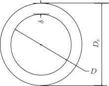
The maximum cavity diameter of Dc is illustrated in Fig. 4. We define the thickness δ of a cavity as

where D is the diameter of the vehicle in the cross section of the maximum cavity diameter. In this study, Dc is determined by examining the contour of the vapor volume fraction, which is illustrated in Fig. 3. The thickness values for various vapor volume fraction regions, which are measured approximately, are listed in Table 1. The thickness will be used to calculate the sound attenuation intensity later.
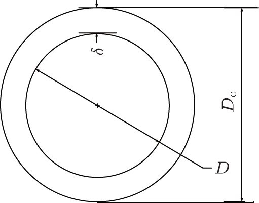 | Fig. 4. Maximum cross section of cavity. |
| Table 1. Thickness values of various vapor volume fraction regions. |
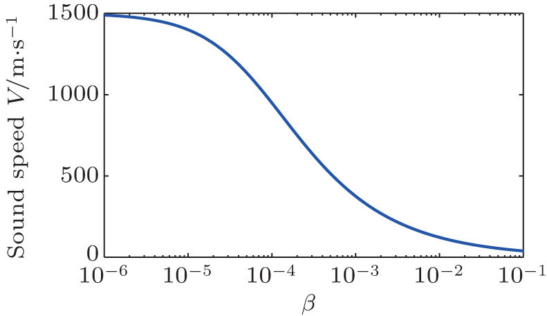
The attenuation coefficient and the propagation velocity of a sound wave are numerically simulated in a bubbly liquid when ω a/c ≪ 1. Values of the physical parameters we used for evaluating Eqs. (49) and (50) are given in Table 2.
| Table 2. Values of the physical parameters used in the model. |
The sound speed changing with the vapor volume fraction at a certain frequency 10 kHz which is far smaller than the resonance frequency can be seen in Fig. 5. The equilibrium radius is set to be 20 μ m. The sound speed decreases with the increasing of the vapor volume fraction. The curve in Fig. 5 has a better agreement with the experiment data which were obtained by Frederick.[21] Figure 6 illustrates the sound attenuation coefficient changing with the vapor volume fraction with the same parameters as those in Fig. 5. With the increasing of the vapor volume fraction, the sound attenuation coefficient increases gradually. Based on the formula of sound attenuation coefficients with various vapor volume fractions, the attenuation of sound intensity will be calculated. The numerical results are listed in Table 3 where the attenuation coefficients are averaged over the corresponding vapor volume faction regions. The overall sound attenuation intensity is 0.607 dB which is sufficiently small so that it can be neglected in engineering.
 | Fig. 5. Variation of sound speed with vapor volume fraction. |
 | Fig. 6. Variation of sound attenuation coefficient with vapor volume fraction. |
| Table 3. Attenuation coefficients and intensities of sound traversing across a cavity. |
In this paper, cavitation around the hemispherical head-form underwater vehicle is simulated and validated with the existing experimental data. The selected cavitation model performs well in the cavitating flows, and the vapor volume fraction distributions around the head are obtained with a large cavitation number. In order to obtain the influence of bubbly liquid on the acoustic wave propagation, the linear wave propagation in bubbly liquid is studied. The sound attenuation coefficient and the sound speed formula of the bubbly liquid are obtained approximately through solving the linearized equation of wave propagation of bubbly liquids and the dynamic equation of bubbles when ω a/c ≪ 1. The results reveal that the sound attenuation coefficient increases as the vapor volume fraction increases. On the contrary, the sound speed will turn smaller. Based on the sound attenuation coefficients with various vapor volume fractions, the attenuation of sound intensity is calculated. The result shows that the sound intensity attenuation is fairly small in a certain condition in this paper. Consequently, the negative effect due to intensity attenuation can be neglected in engineering.
| 1 |
|
| 2 |
|
| 3 |
|
| 4 |
|
| 5 |
|
| 6 |
|
| 7 |
|
| 8 |
|
| 9 |
|
| 10 |
|
| 11 |
|
| 12 |
|
| 13 |
|
| 14 |
|
| 15 |
|
| 16 |
|
| 17 |
|
| 18 |
|
| 19 |
|
| 20 |
|
| 21 |
|