Molecular dynamics simulations are performed with the software NanoMD, ^[19] which is developed by Zhao’ s group (Nanjing University), through improving the models for simulation. The models are [100], [110], [111] nanocubes, whose sizes are all 20a (a denotes the copper lattice constant that is 0.3615  nm) corresponding to 34461, 33341, and 32239 atoms respectively under three-axial tensile loadings (Fig.  1).

Fig.  1.

	Figure Option ViewDownloadNew Window
	Fig.  1. (a) Sketches of nanocubes under uniaxial and three-axial tensile loadings, (b) schematic diagram of crystallographic orientations of three nanocubes under three-axial tensile loadings.

There are tensile atoms whose sizes are a in models, and the tensile atoms without mutual coupling in three directions ensure the independence of tensile loadings in three directions (Fig.  1(a)). Also, there are tensile atoms only in the z direction when the model is loaded under uniaxial tension. Figure  1(b) shows the schematics of three orientations’ models in x, y, and z directions.

In this work, MD simulations are carried out with the embedded-atom method (EAM) potential developed by Johnson, ^[20] which could provide an effective description of the transition metals with a face-centered cubic (FCC) structure. The total energy^[21] is given by

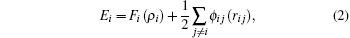
where E_tot is the total internal energy of an assembly of atoms, E_i is the internal energy of atom i, ρ _i is the electron density contribution of all other atoms at atom i, F_i(ρ _i) is the energy to embed atom i into the electron density ρ _i, r_ij is the distance between atoms i and j, ϕ _ij(r_ij) is the pair potential with the distance between atoms i and j being r_ij, and f_j(r_ij) is the contribution of the atom j at r_ij to the electron density at atom i. The potential with the nearest neighbor atom model is used. The pair potential and the embedded energy are given^[22] by

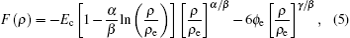
where E_c, ϕ _e, α , β , and γ are the parameters of EAM potentials for FCC metal. The variables with subscript e refer to the equilibrium values of the variables.

During the simulations the number of atoms, the volume and the energy of systems are invariant, corresponding to micro-canonical ensemble in statistical mechanics. The models set 2 × 10⁴ relaxation steps at 30  K at the beginning. The atomic velocity of the models in accordance with Gaussian random number can correspond to the Maxwell– Boltzmann velocity^[23] through relaxation. Then by atomic velocity correction the systems work up to thermal equilibrium states. For stress veracity, when the stresses are all less than 0.01  GPa, the relaxation process stops. After enough relaxation, the tensile atoms of the models are stretched by 0.01%  ps^{− 1} under three-axial tension. The simulation uses a combined Verlet leapfrog and cell-linked list algorithm. Above all, the simulation can reveal some mechanical quantities.

The stress is computed by the virial scheme, and the overall stress is averaged over all atomistic stresses. For the system, the corresponding stress in the n direction is the average stress of the plane atoms, which is perpendicular to the n direction. The corresponding atomic stress is expressed in terms of EAM potential functions as follows:^[24]

where is the ξ η component of the atomic stress tensor of atom i, Ω _i is the average volume of atom i, m_i is the mass of atom i, and are the velocity components in the ξ and η direction of atom i respectively, and are the displacement components in the ξ and η directions of r_ij respectively.

The strain ε is defined as ε = (l − l₀)/l₀, where l is the length of the current model, and l₀ is the length of the model after relaxation. Like the case in macro-mechanics, hydrostatic stress σ _m and Mises stress σ _eq are defined respectively as follows:

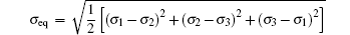
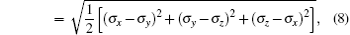
where σ ₁, σ ₂, and σ ₃ are principal stresses, σ _x, σ _y, and σ _z are the stresses in the three directions. Shear stress does not exist, so σ ₁, σ ₂, and σ ₃ can be replaced by σ _x, σ _y, and σ _z.

The Gurson damage model has given four models containing voids, and the model of spherical voids will meet the yield surface equation:^[25]

where σ _s is the yield stress, and h is the volume percentage of the void. When h is a constant value, the equation is the relationship between σ _eq and σ _m because σ _s always is a constant value.

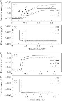
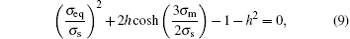
Figure  2 gives the average kinetic energies and potential energies under uniaxial and three-axial tensile loadings. According to thermodynamic kinetic energy formula E_ke = 3/2k_BNT, where k_B, N, and T are the Boltzmann constant, the total number of atoms, and the thermodynamic temperature respectively. The average kinetic energy can be affected only by T. As seen in Fig.  2, the average kinetic energies decrease suddenly and the average potential energies increase with tension increasing after enough relaxation. The average potential energies become different under uniaxial and three-axial tension. Under the three-axial tension, the average potential energies have no obvious secondary peaks (A, B, and C points) (see Figs.  2(a) and 2(b)). The relaxation steps are 20773, 25629, and 26181 steps for [100], [110], and [111] nanocubes. Although this figure is unlikely to be entirely accurate, it can show that the [111] nanocube has bigger stress and enters into the small stress state, and turns harder than the nanocubes of the other two orientations. In other words, the configuration of the [111] nanocube is more difficult to break and more stable than the nanocubes of the other two orientations.

Fig.  2.

	Figure Option ViewDownloadNew Window
	Fig.  2. Average kinetic energies and potential energies of different orientations under (a) and (b) uniaxial and (c) and (d) three-axial tensile loadings.

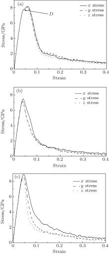
When the [100], [110], and [111] models are under three-axial tension, the different mechanical properties are displayed in three tensile directions. Figure  3 exhibits the stress– strain curves of the models of the three orientations.

Fig.  3.

	Figure Option ViewDownloadNew Window
	Fig.  3. Stress-strain curves of (a) [100] oriented nanocube, (b) [110] oriented nanocube, and (c) [111] oriented nanocube.

All curves exhibit mechanic properties like the macromechanic ones. However, only the [100] nanocube shows the obvious yield stage (D point) and its three curves are almost coincident (see Fig.  3(a)). The x axial curve is different from the other two curves in the [110] nanocube. In the [111] nanocube, three curves are not coincident except in elastic stages. Some detailed mechanical parameters are shown in Table  1.

Table 1.

Table 1.

Table 1. Some detailed numerical values of three crystal orientations in three tensile directions. [100] [110] [111] x[001] y[010] z[100] x[001] y z[110] x y z[111] Yield stress/GPa 8.17025 8.12366 8.11275 7.48015 7.16021 7.12707 8.90265 8.44737 8.42338 Yield strain 0.05943 0.05693 0.05493 0.03947 0.03867 0.03886 0.04705 0.04620 0.04280 Tensile step 5943 5693 5493 3947 3867 3886 4705 4620 4280 Orientation sizea a/2 a/2 a/2 a/2 aOrientation size in the n direction is defined as the projection direction of atoms in the n direction.

Table 1. Some detailed numerical values of three crystal orientations in three tensile directions.

From Table  1, the orientation size affects the yield stress because the stress is given from the statistical average theory. The orientation sizes are similar in the [100] nanocube, so the yield stresses are similar. In the [110] nanocube, yield stress is in proportion to orientation size in the case of ignoring the small error. However, the [111] nanocube is too difficult to forecast the relationship between orientation size and stress because the orientation size is not unique in different planes. Figure  3 shows that in the elastic stage the three stress-strain curves are overlapping in each orientation model. So the Young moduli are similar in the crystal orientation models.

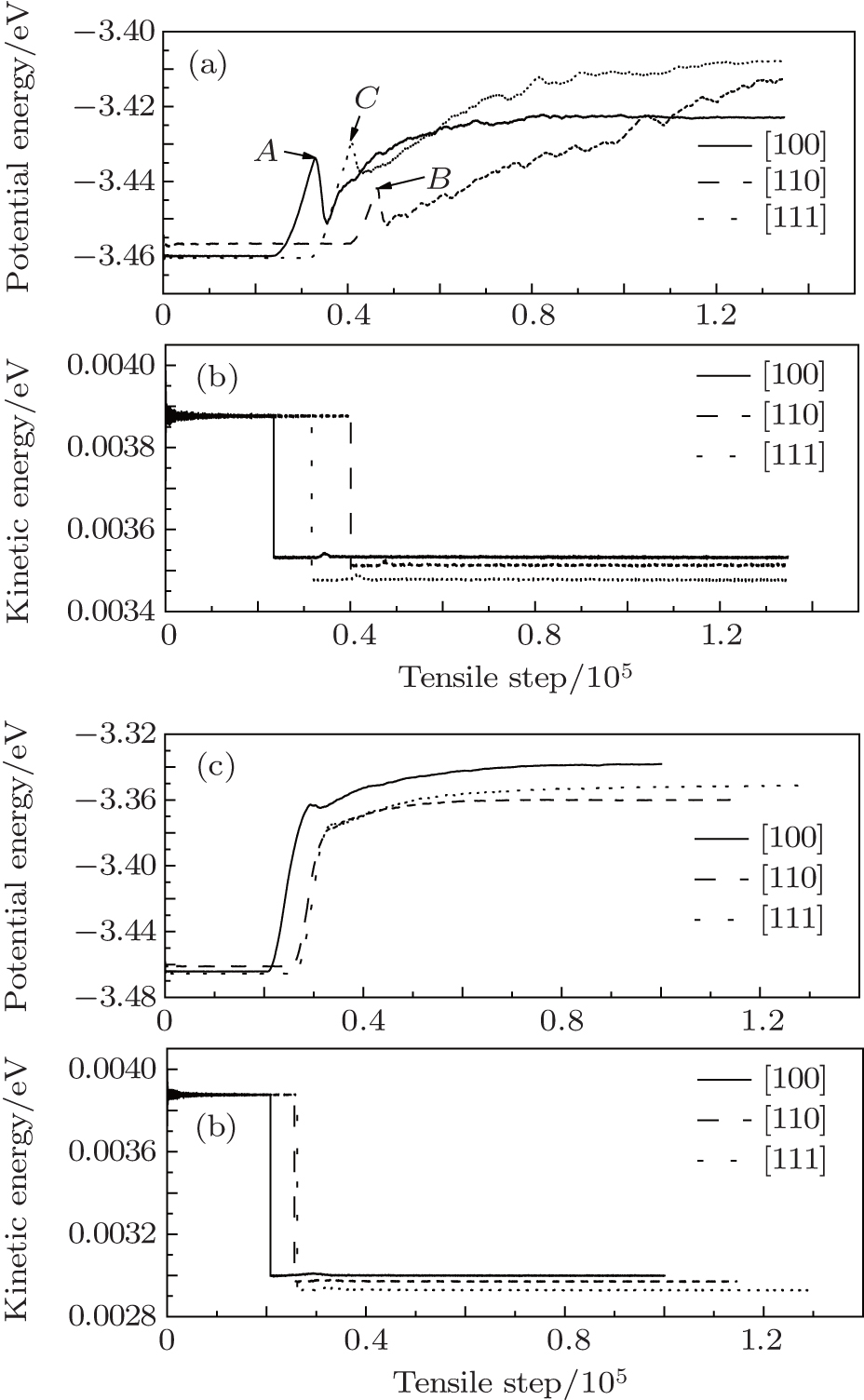
Hydrostatic stress is the stress averaged over the stresses in three directions. Young’ s modulus calculated by the hydrostatic stress– strain curve is about 185  GPa in Fig.  4(a). Mises stress comprehensively considers the influence of the principal stress on the yield strength. Figure  4(b) displays the relationship between Mises stress and strain. With the tensile loadings the Mises stresses first smoothly change then increase quickly, and finally decrease. Like the case in macromechanics, the material also has an elastic stage, yield stage, and fracture stage. The peaks (E, F, G) explain the effect of the orientation size on the stresses in three directions. The hydrostatic stress and Mises stress display the integrity and difference in stress among the three directions.

Fig.  4.

	Figure Option ViewDownloadNew Window
	Fig.  4. Stress– strain curves of nanocubes of different crystal orientations: (a) hydrostatic stress and (b) Mises stress.

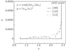
For the Gurson damage model, we need to consider the relationship between the Mises stress and the hydrostatic stress (Fig.  5). When the model has no void, the diagram of y– x should be a straight line. In this case, Mises stress is unrelated to the hydrostatic stress. However, from Fig.  5, it can be understood that only the [100] crystal orientation curve is almost a straight line. The curves are related to not only the void percentage but also orientation sizes. When the hydrostatic stress nearly reaches the yield points, the Mises stress increases more rapidly in the [111] nanocube than the [110] nanocube, and hardly increases in the [100] nanocube. Isotropy is essential to study the microscopic damage.

Fig.  5.

	Figure Option ViewDownloadNew Window
	Fig.  5. Mises stress– hydrostatic stress curves of three crystal orientations.