


A novel simulation method for positive corona current pulses*
[Liu Yang† , Cui Xiang, Lu Tie-Bing, Li Xue-Bao, Wang Zhen-Guo, Xiang Yu, Wang Xiao-Bo]
, Cui Xiang, Lu Tie-Bing, Li Xue-Bao, Wang Zhen-Guo, Xiang Yu, Wang Xiao-Bo]
|
|


†Corresponding author. E-mail: liuyangwuh520@sina.com
*Project supported by the National Basic Research Program of China (Grant No. 2011CB209402), the National Natural Science Foundation of China (Grant No. 51177041), and the Fundamental Research Funds for the Central Universities, China (Grant No. 12QX01).
A novel two-dimensional (2D) simulation method of positive corona current pulses is proposed. A control-volume-based finite element method (CV-FEM) is used to solve continuity equations, and the Galerkin finite element method (FEM) is used to solve Poisson’s equation. In the proposed method, photoionization is considered by adopting an exact Helmholtz photoionization model. Furthermore, fully implicit discretization and variable time step are used to ensure the time-efficiency of the present method. Finally, the method is applied to a positive rod-plane corona problem. The numerical results are in agreement with the experimental results, and the validity of the proposed method is verified.
A number of high voltage direct current (HVDC) transmission lines have been built to meet the large demand on transport of bulk power in China.[1– 3] The corona current pulse on HVDC transmission lines is a predominant source of radio interference, which will interfere with the reception of the amplitude modulated radio. However, due to the complexity of the discharge process, it is difficult to accurately predict the corona current pulses and their radio interference, which is a major obstacle for the pre-design of a new transmission line project.
Since the 1980s, there has been interest to explain the mechanism of corona discharge with numeric methods. In 1985, by assuming that the streamer propagated in a fixed cylindrical channel, Morrow[4] proposed a best-known one-dimensional (1D) model of Trichel pulses. This model has been widely used in subsequent corona studies.[5, 6] However, there are limitations in the applicability of the model due to the errors introduced by the 1D approximation of the space charges.
Later in 2000, Georghiou et al.[7] proposed a full two-dimensional (2D) algorithm to simulate the streamer propagation, which is based on the finite-element method with a flux-corrected-transport technique (FEM-FCT). Though the breakdown voltages predicted by the model were in agreement with the experimental measurements, it should be pointed out that due to the inefficiency of the computation, the simulation was only performed in a 0.2-cm short gap and on a few ns timescale. The restrictions of short gap and short timescale make this method unapplicable to corona current pulse simulations.
In 2007, Ducasse et al.[8] presented a comprehensive comparison of efficiency between the full 2D FEM-FCT and FVM-MUSCL (the finite volume method with monotonic upwind-centered scheme for conservation-law) methods. Both methods were applied to a 1-mm point-plane gap on a 5-ns timescale, and the computation time was 3 h for FEM-FCT and 1 h and 28 min for FVM-MUSCL, which demonstrated the time-consuming characteristic of the two methods.
In 2010, Sattari et al.[9] simulated the corona current pulses with a 2D FEM-FCT approach by considering single ionic species only, with the ionization layer neglected. This simplified treatment greatly improves the efficiency of the simulation. Later in 2011, Sattari and Castle[10] presented a new 2D model, with three ionic species considered, to simulate the Trichel pulses in a 1-cm long point-plane gap. It is worth mentioning that the use of a variable time step technique is very successful in accelerating the computation. The calculated results showed satisfactory agreement with the experimental data. However, the use of explicit discretization for the continuity equation made the Courant– Friedrichs– Lewy (CFL) condition a necessary requirement, resulting in a short time step (∼ 1 ps) and consequent increase of the computation time.
Recently, Yin et al.[11] extended the finite element method with a finite volume method (FEM-FVM) to the simulation of Trichel pulses in a 60-cm long line-to-ground gap. Although their simulation results agreed well with the measurement results, it should be noticed that the corona discharge was assumed to be uniform along the conductor to enable the simulation to be performed in two dimensions. However, the corona discharge is confined to discrete points, which are actually the irregularities located on the conductor surface.[12, 13] Thus, the assumption of a uniform distribution of corona discharge may not be in accordance with the physical nature.
Thus it is seen that a large collection of numerical methods for corona current pulse simulations exists in the published literature. However, none of them is entirely satisfactory in both computation efficiency and physical nature reproduction, which becomes a block for corona current pulses simulations in long gaps and on long timescales. This paper, aiming at clearing this block, presents a method based on the CV-FEM (control-volume-based finite element method)[14] approach. This method is novel in two phases. Firstly, to reduce the tedious computation associated with the 2D continuity equations, a fully implicit discretization technique is adopted to discard the restriction of the CFL condition; furthermore, variable time step technique is taken from previous work.[10, 11] Secondly, the efficient photoionization (important for positive corona) model[15, 16] is first adopted to restore the physical process of corona current pulse production, leading to just a 2.9% increase of computation-cost for the simulation of a 10-cm rod-plane gap; whereas, in previous 2D simulations, photoionization was usually ignored[5, 7, 10, 11] or replaced by a uniform background photoionization[8, 17] for its high computation complexity, which was evidenced as “ the consideration of photoionization costs nearly 90 percent of the computing time in the whole simulation.” [17] The rest of the present paper is organized as follows: firstly, a detailed description of the methodology is presented, which includes the governing equations, boundary conditions, initial conditions, discretization, etc; secondly, the method is applied to a rod-plane example, and a comparison between the simulated results and the measured results is made to verify the validity of the proposed method; thirdly, the convergence of the present method and the physical implications of the results are discussed; finally, some conclusions are derived.
To clearly describe the essential ingredients of the proposed methodology, a rod-plane corona problem is taken as
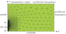
 | Fig. 1. Configuration of calculation domain. |
the context. Figure 1 shows the configuration of the rod-plane electrode system, which consists of a rod anode and a plane cathode. The electrode gap is 10-cm long. Owing to the axisymmetric property of the problem, an axisymmetric cylindrical coordinate system, ρ – z, is used.
Despite the complexity of the physics associated with the corona discharge, some basic processes involved in corona have been revealed through the efforts of many investigators. It is now an acknowledged fact that the basic processes of corona discharge are collision ionization, photoionization, attachment, recombination, diffusion, and drift.[18] Considering all of the specific particles and the relevant reactions in the corona discharge will be a great challenge.[19– 23] In order to simplify the present investigation, the widely-used hydrodynamic model[4– 11, 17, 19– 25] which takes the aforementioned basic processes into account is adopted. The governing equations of the hydrodynamic model are


where

In Poisson’ s equation (1): φ denotes the electric potential; Ne, Nn, and Np represent the number densities of electron (e), negative-ion (n), and positive-ion (p), respectively; ε 0 is the permittivity of air; and e is the absolute value of the electronic charge. In the continuity equation (2): t is the time; Js is the current density; the subscript “ s” refers to the three ionic species, i.e., e, n, and p; υ denotes the drift velocity; D is the diffusion coefficient, and it is set to be zero for positive and negative ions due to the lower efficiency of their diffusion; and S is the source term due to ionization, attachment, recombination, and photoionization. All the transport coefficients of air are listed in Appendix A.
The boundary conditions for Eq. (1) are that[8] on the anode surface, φ is set as the applied voltage; on the cathode surface, φ = 0 is applied. The boundary conditions for Eq. (2) are that at the anode, a Neumann condition ∂ N/∂ n = 0 is applied for Ne, whereas Np is set to be zero; at the cathode, Nn and Ne are both set to be zero.
The initial conditions for Eq. (2) are that to trigger the avalanche, a neutral plasma spot of Gaussian form is set to be in the calculation domain. The initial distribution of the neutral plasma in the present problem is expressed as
where N0 = 1.0× 10¹⁰/m3, z0 = 9 cm, and s0 = 25 μ m. Simulation shows that different values of the parameters in Eq. (4) will not change the waveform.
To restrict the calculation in a finite domain, an artificial boundary is selected which is far from the tip of the anode to avoid the influence of space charge. At the artificial boundaries, a Neumann condition is applied to electric potential φ and electron density Ne. The coupled 2D equations (1) and (2) are solved on a nonuniform mesh, which has very fine spatial resolution in the region close to the tip of the anode, while it has very coarse but adequate resolution far from the discharge region. Poisson’ s equation is solved with the Galerkin finite element method (FEM); whereas the continuity equations are solved with the CV-FEM. The flow chart of the algorithm is shown in Fig. 2 where T denotes the timescale of the simulation, and Δ t denotes the time step.
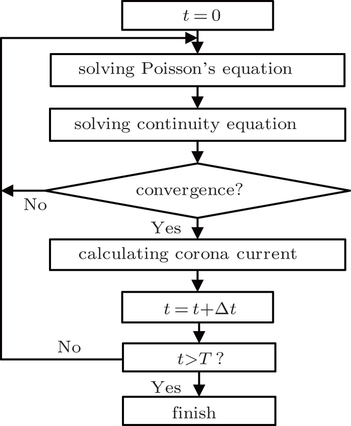 | Fig. 2. Flow chart of the algorithm. |
In the present scheme, fully implicit discretization is applied. Thus, to calculate the density at a given time level, the parameters such as ionization coefficient, diffusion coefficient, and mobility coefficient should be updated to the values at the present time level. However, only the coefficients at the last time level are known. In order to obtain the accurate solutions, iterative calculations between Eqs. (1) and (2) are needed at each time step as shown in Fig. 2.
Galerkin’ s FEM formulation of Eq. (1) over an element can be cast into the following form:

where Ω e is the domain bounded by the element of interest; 


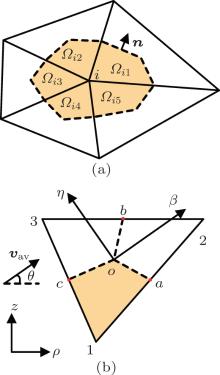
Following the triangular mesh of the calculation domain, the node centered volumes can be formed by joining the centroids of elements to the midpoints of the corresponding sides. Figures 3(a) and 3(b) show a control volume and a typical triangular element, respectively. The solid lines denote the element sides, and the dashed lines represent the control-volume faces. An integral formulation of Eq. (2) over a control volume, say Ω i (control volume surrounding node i), reads

where ∂ Ω i is the boundary of the control volume Ω i, n is a unit vector outward normal to the control volume face, dτ denotes the infinitesimal quantity for the length of the control volume face and here the subscript “ s” in Eq. (2) is omitted for conciseness. Figure 3(a) shows that the control volume Ω i can be seen as a combination of several sub-control-volumes, which are denoted by Ω ij (j = 1, 2, … , M, M is the number of sub-control-volumes surrounding node i). The symbol υ av in Fig. 3(a) denotes the average value of υ over the element of interest. In order to formulate the algebraic expressions of Eq. (6) in an element-by-element procedure, equation (6) is rewritten in a form of summation of the contributions from all the associated elements of node i as follows:

where ∂ Ω ij are the control faces associated with the sub-control-volume Ω ij.
The element-average values of ρ , D, S, and υ are stored, and they are assumed to prevail over the corresponding elements. In the following context, the discretization of Eq. (7) will be presented by taking the element shown in Fig. 3(b) for example, and node 1 is chosen as the node of interest. Points a, b, and c are midpoints of the corresponding sides of the triangular element.
 | Fig. 3. Details of the discretization and relevant quantities for the continuity equations: (a) control volume of node i, (b) a typical triangular element and its key points for construction of the discretization. |
The integral involving the unsteady term is approximated as follows:

where A is the area of the triangular element, ρ av is the element-average value of ρ , 

As the transport of ionic species in corona discharge is a convection– dominated diffusion problem, linear interpolation of number density N will cause physically unrealistic oscillations.[14] The upwind scheme is therefore adopted in the present method to cope with this problem. In order to construct the upwind interpolation function of N, it is useful to define a particular new β – η coordinate system for each element as shown in Fig. 3(b). Its origin is located at the centroid o, and the β axis is aligned with the element-average velocity υ av, while the η axis is perpendicular to υ av. The transformation between the ρ – z and β – η coordinate systems can be performed through
where θ denotes the angle between the ρ axis and υ av. The discretization of the integral of the convection– diffusion term over the sub-control-volume 1aoc can be written as

where Dav is the element-average value of D, lao⊥ is the distance from centroid o to side 12 where point a is located, and lco⊥ is the distance from centroid o to side 13 where point c is located.
The integral involving the source term is approximated as follows:

where 
The conditions for continuity equations can be classified into two categories: one is the Dirichlet condition (at the inflow boundary, N = 0), and the other is the Neumann condition (at the outflow boundary, ∂ N/∂ n = 0) as shown in Fig. 4. The Dirichlet condition is applied by just setting the unknowns at the boundary nodes to be the specified values. As for the Neumann condition, each of the unknowns at the boundary nodes are set to be the average values at their adjacent upwind nodes. For example, N1 = 0.5N2 + 0.5N3 is applied to node 1, which is a simple but good approximation to the Neumann condition since the straight line determined by node 1 and the midpoint of node 2 and node 3 is almost aligned with the normal direction of the outflow boundary.
According to Eqs. (8), (10), and (11), the contributions to the continuity equations from all the sub-control-volumes surrounding node 1 are obtained similarly. Adding up all the contributions yields the discretization equation for node 1. With the same procedure performed over all the nodes, a system of linear equations is obtained. Applying the boundary conditions to the linear equations gives the discretization equations for the continuity equations.
In all the integrals that do not involve the unsteady term, the values of N at time level m are used, resulting in a typical fully implicit discretization, which is free of stability restrictions on the time step.
 | Fig. 4. Illustration of the boundary conditions for a typical convection-diffusion problem. |
By fitting the absorption function with a series of exponents, the photoionization term can be divided into three components 

where λ j and cj are the coefficients determined by the fitting. A three-exponential fitting is applied to the absorption function, and the coefficients of the fitting are cited from Ref. [16]. Equation (1) can be seen as a special case of Eq. (12) with λ set to be 0. The resulting Galerkin FEM discretization of Eq. (12) reads

The matrices K1 and K2 are shared by Eqs. (1) and (12), so no extra computation is introduced by photoionization. The matrix K1 − K2λ can be inverted and stored at the beginning and then only a multiplication is needed to solve the linear system (13) at each iteration. It is found that photoionization consumes just 2.9% of the whole computation time in the present model (it takes 0.064 s for one iteration of 2.20 s).
To determine the solution of Eq. (12), it suffices to define the boundary condition, and thus zero boundary condition[15] is enforced in the present method.
Because of the high velocity of electrons during corona discharge, a short time step is necessary to ensure a fast convergence, and otherwise a long time step means a large Courant number, which will consequently slow down the convergence or even cause a divergence. This restriction becomes intolerable especially in the case of a long timescale simulation such as a current pulse train simulation, which is unfortunately just the subject of this paper. Therefore, it is urgent to find a technique which can improve the way of using the time step.
During the corona discharges, a lot of electrons will be produced and consequently corona current pulse arises due to their rapid motions. In this pulse stage, electrons play a predominant role and thus in any case cannot be ignored, and a short time step should be used. However, after the corona is extinct, the majority of electrons are absorbed by the anode in a short time and a few of them will attach to molecules to form negative-ions, and what succeeded is a long time, which is necessary for the dispersion of the positive ions.[18] During this long time, i.e., the steady stage, there are only a small number of electrons and therefore the effect of electrons can be ignored, which makes it possible to use the long time step at this stage. The aforementioned facts constitute the theoretical basis of the technique of variable time step, [10, 11] the implementation of which is to use a short time step at the pulse stage and a long time step at the steady stage. Since the mobility of the electrons is at least 100 times larger than the mobility of the ions, the time step is 1 ns for the pulse stage (electron-dominated) of the current, whereas 100 ns for the steady stage (ion-dominated) in the present simulation.
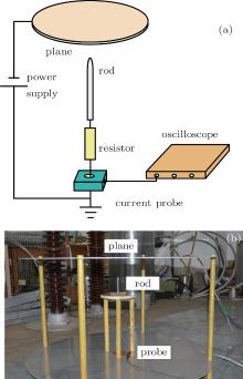
An experimental setup with a rod-plane gap shown in Fig. 1 is built to verify the proposed method. Figure 5 shows
 | Fig. 5. Experimental setup for positive corona: (a) sketch map, (b) photograph. |
the experimental setup where the negative voltage is applied to the plane electrode, whereas the rod electrode is connected to the ground through a resistor. The rod electrode is positive with respect to the plane electrode and thus positive corona discharge will occur at the tip of the rod electrode.
Figure 6 shows the comparison between the simulated results and the measured results at a voltage of 30 kV. As shown in Fig. 6(a), both the measured pulse and the simulated pulse show similar shapes, which first increase rapidly and then decrease somewhat slowly, although the simulated pulse has a shorter duration than the measured pulse. Due to the random nature of corona discharge, peak values of the pulses fluctuate, and there are random intervals between the pulses, as shown in Fig. 6(b). However, the simulated pulse train shows similar behaviors to the measured one.
 | Fig. 6. Results comparison among (a) single pulse, (b) measured pulse train, (c) calculated pulse train. |
Complete identity of simulated results and measured ones is desirable but difficult to achieve since the corona discharge is an extremely complex phenomenon which appears quite different under various environmental conditions and the coefficients used in the simulation may not accurately characterize the practical environmental condition, in addition, some random factors cannot be considered in the simulation. For the mentioned reasons, it is believed that the similar pulse shape and similar time distribution pattern of the two results indicate the validity of the proposed method.
The time efficiency and the convergence of the proposed method as well as the physical implications of the results are discussed in the following.
To evaluate the time efficiency of the proposed method, simulations are performed with the proposed method as well as the previous method FEM-FCT. For the sake of fairness and objectivity, the time consumption in one time step simulation is chosen as the indicator of the time efficiency. Applying both methods to the same simulation (using the same mesh, the same computer, and the same programming skills) gives the result: the time consumption is about 2.20 s per time step for the proposed method and about 3.28 s for FEM-FCT. It can be seen that the proposed method has a higher time efficiency than FEM-FCT.
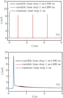
The convergence is one of the most important aspects for a numeric method, and thus it is necessary to check the convergence of the proposed method. For this purpose, the time step strategy is changed to restart the simulations and to see whether the results given above converge or not. Two other time step strategies are used to check whether the time step strategy used above is able to ensure a converged result. The time step strategy used above has variable time steps of 1 ns and 100 ns. The two other time step strategies are variable time steps of 1 ns and 200 ns, and a constant time step of 1 ns. Secondly, another finer mesh is adopted to check whether the mesh used above is fine enough. The number of nodes in the above mesh is 2507, while the number of nodes in another mesh is 3732.
The results obtained when using different time step strategies are shown in Fig. 7. The figure indicates that the waveforms obtained with applying variable time step strategies are almost the same as those obtained with a constant time step of 1 ns, except for a little error in the steady stage of the pulses. This error is due to the difference of the time step used during the steady stage of the pulse. However, figure 7 indicates that the error is negligible, which means that the results when using the variable time steps of 1 ns and 100 ns converge well in the time step.
Figures 8(a) and 8(b) show the results under 2507-node mesh and 3732-node mesh, respectively. Both results show the same feature, namely, the first pulse has a large peak value; as the simulation goes on, the pulses show regular peak values and time intervals. It is important to note that only the pulses during the simulation becoming steady can well represent the real scenarios occurring in a corona discharge. The reason is that to trigger the electron avalanche, an initial space charge distribution is specified. However, the specified initial space charge distribution possibly does not appear during the corona discharge, and thus the first few pulses possibly cannot represent the actual situations.
Figure 8 indicates that when the simulation is steady, the results under both meshes are basically the same: under 3732-node mesh, the peak value of the pulse is about 10.58 mA, time interval is about 1.77 ms; whereas under 2507-node mesh, the peak value of the pulse is about 9.54 mA, time interval is about 1.67 ms. As a result, if the results under 3732-node mesh are taken as the reference, the relative error of the peak value is 9.83% , and that of the time intervals is 5.65% . It follows that the results under 2507-node mesh are close to the results under finer meshes and hence it is believed that the results given in Section 3 converge well in element size.
 | Fig. 7. Results comparison among different time steps for (a) pulse train, and (b) enlargement of the first pulse. |
 | Fig. 8. Results under (a) coarse mesh with 2507 nodes, and (b) fine mesh with 3732 nodes. |
As shown in Fig. 6(a), the corona current pulse has a steep rising edge, subsequently a relatively slow falling edge, and finally a long trail. The following discussion is about the physical implications of the waveform at different stages.
The corona current pulse is due to the motion of the electrons and ions. The Shockley– Ramo Theorem[18] states that the current induced by the moving charge is proportional to the velocity of the moving charge. The velocity of electrons for a given electric field is generally two or three orders of magnitude higher than that of ions, thus, the motion of electrons will contribute to a higher-amplitude but a shorter-duration current; the current due to the motion of ions is of a lower-amplitude but of a longer-duration. Therefore, the motion of electrons plays a predominant role in the rising stage and falling stage of the pulse, whereas the long trail is caused mainly by the motion of ions.
A complete corona pulse can be divided into three stages. The first stage is the rising stage. The positive ions left by preceding corona discharges are expelled far from the anode before the next discharge can take place, so at the beginning stage of a corona discharge, the condition is in favor of the avalanche development, [13, 18] and thus resulting in a rapid increase of the current. The second stage is the falling stage. During the corona discharge accompanying the primary avalanche, a lot of secondary avalanches are initiated by the electrons produced by photons, and thus the pulse will last for a period of time. Meanwhile, it should be borne in mind that with a lot of avalanches being formed, a lot of positive ions will be produced and accumulate in the space, thereby causing an increasing suppression effect on the avalanche development, consequently the current begins to decrease and show a falling edge. The third stage is the trail stage. The increasing suppression will finally cause the extinction of the avalanche activities and then the current will be totally caused by the motion of positive ions and minor negative ions. Also by applying the Shockley– Ramo Theorem, this ion-motion-caused current will decrease as the positive ions continue to move away from the anode. The velocity of positive ions decreases during its motion and thus the clearance of positive ions will need a long time, thereby causing the current to have a long trail.
A novel 2D CV-FEM method is applied to a 10-cm rod-plane gap on about a 10-ms timescale, and the simulation results are compared with the experiment results. According to the analyses and discussion, the conclusions drawn from this work are as follows.
(i) Variable time step techniques and fully implicit discretization greatly improve the efficiency of the method. The time step is 1 ns for the pulse stage (electron-dominated), 100 ns for the steady stage (ion-dominated), which is quite a lot larger than the time step used in the previous explicit methods.
(ii) An efficient Helmholtz photoionization model is introduced into corona current pulse simulation. The calculation for photoionization takes only 2.9% of the whole computation time.
(iii) An experiment is carried out to verify the validity of the proposed method, and the simulated results and measured results are in agreement in the sense of the pulse shape and time distribution pattern.
(iv) Electron motion is a predominant reason for causing the rapid rising stage and falling stage of the pulse; the positive ion motion is the main reason for producing the long trail of the pulse.
The authors are much indebted to Dr. Zhuang Chi-Jie and Dr. Yin Han for their guidance and advice during the scheme designing and programming.
| 1 |
|
| 2 |
|
| 3 |
|
| 4 |
|
| 5 |
|
| 6 |
|
| 7 |
|
| 8 |
|
| 9 |
|
| 10 |
|
| 11 |
|
| 12 |
|
| 13 |
|
| 14 |
|
| 15 |
|
| 16 |
|
| 17 |
|
| 18 |
|
| 19 |
|
| 20 |
|
| 21 |
|
| 22 |
|
| 23 |
|
| 24 |
|
| 25 |
|