Near-wall quasi-stream-wise vortices play a key role in producing high friction in the wall-bounded turbulent flow.^{[1– 8]} Aiming at skin-friction reduction and turbulence suppression, the opposition control was proposed by Choi et al.^[9] in their direct numerical simulation (DNS) for the first time.^{[10– 15]} However, it is impractical since the required velocity information very near the wall is usually unavailable. For practical implementation, the suboptimal control scheme by Lee et al.^[16] only used the measurable information about the wall such as the wall pressure. In the wall-bounded turbulent flow, the wall pressure fluctuation field is closely related to the non-stationary motion of turbulent eddies. Poisson’ s equation for incompressible flow,

shows that the wall pressure, p, is influenced by the velocity u (u_i and u_j are the components of u) in the entire boundary layer.

The wall pressure fluctuation, p′ , beneath the turbulent boundary layer (TBL) has been studied since the 1950s.^{[17– 22]} Experimental studies on p′ have been reviewed by Willmarth^[23] and Bull.^[24] Because of its very small amplitude and relatively wide frequency range, it is still a challenge to measure p′ accurately in an experiment. For traditional measuring techniques, such as the electronic pressure scanner valve and pressure sensitive paint, poor performances in the high-frequency response hardly meet the requirements of multi-scale analyses on p′ . To capture high frequency spectra and to enhance spatial resolution, a sufficiently small pressure transducer is desirable.^{[25– 27]} Microphones with a wide frequency-response range, high pressure resolution, and small size perform satisfactorily in our experiment. On the other hand, the hot wire anemometry (HWA) in the TBL, which has been used for several decades, shows that the precision of measurement near the wall is due in large part to the hot wire probe used.^{[28– 30]} Unlike a common straight probe, a miniature boundary layer probe can minimize interference in the flow field and allow fine measurements of velocity very close to the surface.

In this paper, we use microphones and a miniature boundary layer probe to carry out the measurement of weak wall pressure fluctuation p′ and stream-wise velocity u respectively. A set of experimental data on u and p′ in the TBL is attained with the same Reynolds number. We attempt to address the relationship between p′ and stream-wise velocity fluctuations u′ by examining the power spectral density (PSD) and the transfer function, which is the PSD ratio of u′ to p′ . It is conducive to the simplification of TBL control strategy from opposition control to sub-optimal control. Wavelet analysis reflects the time-frequency evolutions and the multi-scale natures of u and p′ . Some comparisons between Fourier transfer and wavelet transfer are also included.

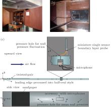
Experiments were conducted with the temperature kept constant in an annular-return wooden wind tunnel in the fluid mechanics laboratory at Tianjin University. The flow developed along one side of a flat acrylic glass plate that was mounted vertically in the wind tunnel. The leading edge of the plate was processed into a half-oval shape. The external and internal views of this wind tunnel are shown in Figs. 1(a) and 1(b). Following the right-hand rule, the space coordinate system Oxyz is set with O as the origin at the leading edge of the plate, x as the stream-wise direction, y as the span-wise direction, and z as the wall-normal direction.

Fig. 1.

	Figure Option ViewDownloadNew Window
	Fig. 1. (a) External view and (b) internal view of an annular-return wooden wind tunnel; (c) schematic diagram of the experimental set-up.

There are 4 holes at x = 71, 92, 113, and 134 cm in the plate, each with a diameter of 1 mm. To achieve a TBL with zero-pressure-gradient along the x direction, which is the object of our experimental study, the pitch angle of the plate was adjusted carefully. We measured the mean wall pressure through the 4 holes by using an inclined tube micro-manometer with a resolution of 0.10-mm H₂O. Three pressure differences between adjacent holes were attained. The root mean square (RMS) of pressure difference was less than 3.4‰ of free-stream dynamic pressure q, which implies that the TBL flow was under nearly zero-pressure-gradient.

A piece of twisted-pair wire was fixed span-wisely at x = 8 cm and then 4 pieces of No. 240 sandpaper were attached along the wire until x = 53 cm. These measures accelerated the transition of boundary layer^{[31– 33]} and made us achieve the fully developed TBL flow at x = 1090 cm where velocity and wall pressure fluctuations were measured respectively. This could be confirmed by the mean stream-wise velocity profile described in the section of flow field validation.

The stream-wise velocity components of u in the TBL were elaborately measured by the constant temperature HWA of an IFA-300 with a miniature single sensor boundary layer probe, TSI-1621A-T1.5. The probe provides a protective pin to allow measurements close to the surface and a long radius bend to minimize disturbances, as seen in Fig. 1(c). The hot wire of this probe is made of tungsten (platinum coated) with a sensitive area length of 1.25 mm and a diameter of 4 μ m. Before velocity measurement, mean-flow calibration was performed by an air velocity calibrator model 1127 of the IFA-300. Calibration was repeated at least twice in order to acquire the best relation between bridge voltage and fluid velocity. The calibration error was 0.087% based on the 4th order polynomial curve fitting. A computer controlled traverse system helped us carry out the velocity measurements at 161 unequal-interval wall-normal points. The separation between adjacent gauging points was 0.02 mm near the wall and 5 mm away from the wall. We set the sampling rate and low pass cut-off frequency to be 100 kHz and 50 kHz respectively according to the forecast about the integral scale and Taylor differential scale. The low pass filter could avoid aliasing problems and remove unwanted high frequency electromagnetic noise to gain a signal-to-noise ratio (SNR) up to 60 dB/decade. Time sequences of u were finally achieved and each sequence consisted of 2²² moments in about 42 s.

In the rectangular accessory of 10 mm in thickness, there was a through hole with unequal sections prepared for the measurement of p′ . The upper surface of the accessory was kept flush with the plate surface. As seen in Fig. 1(c), the upper pin-hole was 5 mm in depth and 1 mm in diameter. It could help to improve the spatial resolution. The lower portion of the hole had a diameter of 6 mm. The electret condenser microphone had a diameter of a little less than 6 mm and a thickness of 3.5 mm. It was placed into the hole to keep lower surfaces of the accessory and microphone flush. The Helmholtz resonant frequency of the pin-hole and cavity is about 3.1 kHz. The sensitive surface of the microphone can feel p′ transmitted through the pin-hole and cavity. An HS6020A sound level calibrator was used to calibrate the relation between system output voltage signal and p′ . Under a sound level of 94 dB corresponding to RMS pressure fluctuation Pa, we conducted the standard-deviation calibration 3 times. The sensitivity of the pressure measurement system is 8.905 Pa/V (the ratio of pressure fluctuation to output voltage) with a reproducibility of 97.2%. The sampling rate was 20 kHz. We attained 100 blocks of p′ signals, and each block was a time sequence of 2 × 10⁴ time points.

In the present experiment, the free stream velocity U_∞ in the test section is 9.59 m/s with turbulence level less than 1%, and is the RMS value of free stream velocity fluctuation. The basic flow field properties of the TBL are listed in Table 1. The nominal thickness δ of the TBL is 39.88 mm at the measuring location x = 1090 mm. This corresponds to Re_θ = 2519 based on the momentum thickness θ and free stream velocity U_∞ . The momentum thickness θ is expressed as dy, and the displacement thickness δ * is expressed as dy. The measured shape parameter H of 1.35, i.e., δ * /θ , implies that the TBL flow represents a reasonable approximation to an equilibrium state^{[34, 35]} and the adjustment for nearly zero-pressure-gradient is effective. The skin friction velocity u_τ is estimated by means of regression of logarithmic law u⁺ = (1/κ )ln y⁺ + C, where κ = 0.40, C = 5.5, between y⁺ = 57 ∼ 142 (defined later). u_τ corresponds to a skin friction stress and a friction coefficient . For the incompressible flow in our experiment, the density ρ of air flow is 1.292 kg/m³ with taking into consideration the environment temperature of 21 ° C and the atmospheric pressure of 101.5 kPa.

Table 1.

Table 1.

Table 1. Basic statistic properties of the TBL flow. U∞ /(m/s) 9.59 H = δ * /θ 1.35 uτ /(m/s) 0.396 Re = U∞ δ /ν 24092 uτ /U∞ 0.0413 Reθ = U∞ θ /ν 2519 δ /mm 39.88 Reτ = uτ δ /ν 996 δ * /mm 5.63 0.2026 θ /mm 4.17 0.00341

Table 1. Basic statistic properties of the TBL flow.

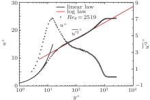
Figure 2 shows the measuring results of the mean longitudinal velocity profile scaled with inner variables (u_τ and ν , ν is the kinematic viscosity coefficient). The measurement results are in good consistency with exemplary curves of the linear law u⁺ = u/u_τ = yu_τ /ν = y⁺ at y⁺ < 5 and the logarithmic law at 50 < y⁺ < 200. The buffer layer 5 < y⁺ < 50 and the wake region 200 < y⁺ < 1000 are also presented as expected.

Fig. 2.

	Figure Option ViewDownloadNew Window
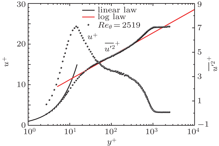	Fig. 2. Profiles of mean longitudinal velocity and Reynolds normal stress.

Hot wire sensors act as spatial filters with a low-pass cut-off frequency, which is dependent on its length. The miniature single sensor whose length is l⁺ = 31 in inner scaling owns sufficient spatial resolution, according to the probability density function of the streaks’ span-wise spacing.^{[28, 30]} Coupled with a ratio of sensor wire length to diameter (l/d) of 312.5, the frequency response of this sensor wire is guaranteed and its dependence on support-stub conduction and eddy-averaging effects could be ignored. The mean profile measured seems to be acceptably accurate even down to y⁺ = 2.7.

The wall-normal distribution of Reynolds normal stress component scaled with is also presented in Fig. 2. A peak of at y⁺ = 14 shows the most intensive turbulent motion in the buffer layer. The peak also reflects the precision of present velocity measurement to a certain extent.^{[36– 39]} In the wake region, the profile of manifests as the ‘ Shoulder’ shape and attenuates abruptly to the free stream turbulence level.

The third and fourth moments of u′ plotted against y⁺ are presented in Fig. 3. In the viscous sub-layer, skewness is positive with a value as high as 1.1 at y⁺ = 2.7. There is intermittency in the u′ signal as suggested by a value of 4.8 for kurtosis at y⁺ = 2.7. The skewness and kurtosis monotonically decrease to − 0.12 and 2.4 at y⁺ = 26.7 and y⁺ = 14.2 respectively. Then they both rise to connect with the log law region. The skewness and kurtosis in the log region are approximately zero and three respectively. This quasi-Gaussian distribution is strict in the range 50 < y⁺ < 200. Beyond y⁺ = 200, the skewness begins to decrease, while the kurtosis begins to increase later. Two opposite sharp peaks indicate the tremendous variation of skewness and kurtosis, which is caused by the wake region with strong intermittency.

Fig. 3.

	Figure Option ViewDownloadNew Window
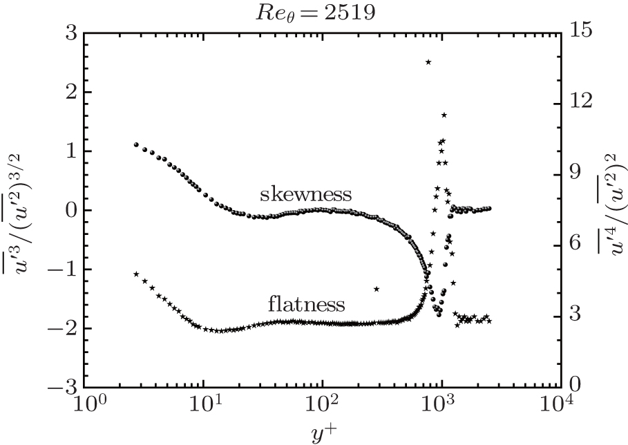	Fig. 3. Distributions of skewness and kurtosis.

The probability density functions (PDFs) of at y⁺ = 5.2, 15.5, 51.7, and 621, are attained by using kernel smoothing density estimation, and the PDF curves in linear and log scale are shown in Fig. 4. The distributions perform as anticipated by Fig. 3. The PDF of is also presented in Fig. 4. Although it approximates to Gaussian distribution: there are 2 longer wings beyond as shown in Fig. 4(b). The flatness of 3.456 also implies this weak intermittency. Some other statistic results of p′ are listed in Table 2. The skewness of 0.006 indicates the good symmetry of p′ . The dimensionless coefficient of divided by the skin friction stress τ _w is 3.06. This result is a little larger than the predicted quantity of 2.92 from the following equation given by Farabee and Casarella:^[19]

Fig. 4.

	Figure Option ViewDownloadNew Window
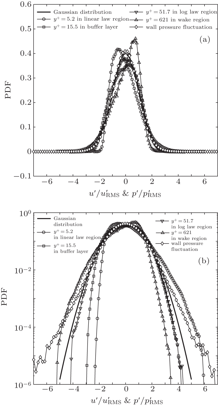	Fig. 4. PDFs of and (a) in linear scale and (b) in semi-log scale.

The scatter is pertinent to the configuration of the pinhole microphone.^{[20, 35]}

Table 2.

Table 2.

Table 2. Statistic properties of wall pressure fluctuation p′ .

Table 2. Statistic properties of wall pressure fluctuation p′ .

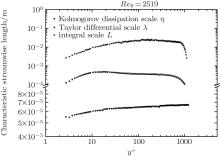
There are three kinds of typical spatial scales in the multi-scale turbulent system. The Kolmogorov dissipation scale η indicates that the fluctuating kinetic energy is transformed into thermal energy by the viscous molecular movement. The Taylor differential scale λ is the length scale of the smallest scale eddies that are produced and identifiable. The integral scale L reflects the spatial dimension of the turbulent fluctuating structure, on the order of the mean motion scale.^[40] Before acquiring Kolmogorov scale η = (ν ³/ε )^1/4, we calculate the mean turbulent kinetic energy dissipation rate, where is inferred from the experimental value of by using Taylor’ s frozen hypothesis with local mean velocity u as the convection velocity.^{[37, 41, 42]} The latter two kinds of scales λ and L are achieved through autocorrelation analysis and Taylor’ s frozen hypothesis as follows:

where is the autocorrelation coefficient of longitudinal fluctuating velocity temporal sequence u′ (t). As shown in Fig. 5, the three kinds of scales have relatively stable values: η ∼ 10^{− 5} m, λ ∼ 10^{− 4} m, and L ∼ 10^{− 2} m in most regions of the TBL, respectively. Compared with Kolmogorov scale η , the sensor wire with the 4-μ m diameter is thin enough to identify the multi-scale system of the whole TBL. Integral scale L keeps the same order of magnitude as δ of the TBL. The corresponding characteristic times of η and λ are both rather larger than 2 × 10^{− 5} s, which proves out the settings of sampling frequency and low-pass frequency.

Fig. 5.

	Figure Option ViewDownloadNew Window
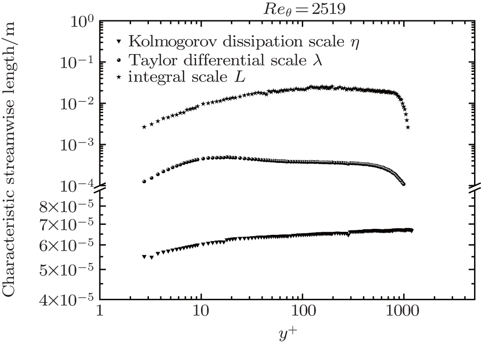	Fig. 5. Distributions of typical spatial scales η , λ , and L.

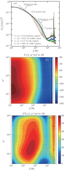
We use the Bartlett method based on fast Fourier transformation to obtain the power spectra of u′ at different values of y⁺ and p′ . The curves of versus frequency f at y⁺ = 5.2, 15.5, 51.7, and 621 are presented in Fig. 6(a). These wall-normal locations are selected specially in different sub-regions of the TBL. With , the area under each curve is 1.

Fig. 6.

	Figure Option ViewDownloadNew Window
	Fig. 6. (a) Spectrum curves of u′ at different values of y+ with exponential scaling laws; (b) distribution of Fu(f, y+ )df in plane (f, y+ ); (c) distribution of f2Fu(f, y+ )df in plane(f, y+ ).

There is widespread agreement with the energy cascade in homogeneous flows with the Reynolds number high enough, and so it is in wall-bounded flows at a certain distance from the wall. According to the classical theory, the frequency domain of the spectrum can be divided into 3 parts, i.e., the energy-containing range, inertial sub-range, and viscous dissipation range. The dimensional analysis by Heisenberg

suggests the − 5/3 law in the inertial sub-range of f ≪ f_s, and the − 7 law in the viscous range of f ≫ f_s. Here, f_s is a frequency in the intermediate range where inertial force and viscosity both play a role, and is of the same order of magnitude as the Kolmogorov scale.

The trend in going away from the surface before the wake region is to have more energy in the frequency range where the viscosity predominates. Another noticeable point is that f_s becomes larger as y⁺ increases. These two phenomena are both due to the non-isotropy caused by the wall boundary. It becomes weaker as y⁺ increases, and there would appear a marked range of local isotropy, which is accompanied with the extensive inertial sub-range and contains the energy viscous range. Compared with it in the log law region, the high-frequency content in the wake region decreases slightly. It is a larger-scale intermittent structure in the wake region that leads to this difference. The wall-normal location determines the spanning sizes of each sub-range in the cascade, which affects whether an eddy can be considered to be viscous, or inertial.^[43]

Figure 6(b) shows the shaded contour of F_u(f, y⁺ )df in dB. Each horizontal section is a power spectral function at a given wall distance. This representation clearly shows the evolution of energy in the whole TBL. The high-frequency wing of the inner peak is captured in the power spectra contour. The wall-normal location of the inner peak at y⁺ = 14 is evident.

The shaded contours of f²F_u(f, y⁺ )df in dB are presented in Fig. 6(c). The second moment spectrum is proportional to an estimate of the turbulent dissipation rate . The evident peak of ε at (y⁺ = 20.5, f = 439 Hz) is located in the dark part of a ribbon. This dark part is related to the near-wall effects, while the other part of the ribbon is dependent on Re_τ . This ribbon topology with an inflection point at about y⁺ = 80 is consistent with the surrogate vorticity dissipation.^[43] According to Taylor’ s frozen hypothesis and the relationship between Fourier transformation and autocorrelation, the Taylor scale λ can also be achieved by

There is good agreement with the results in Fig. 5. Comparing Fig. 6(c) with Fig. 6(b), it can be concluded that the eddies related to turbulent dissipation are about one order of magnitude smaller than the energy-containing eddies with Re_τ = 996. Meanwhile, their peaks are both located in the buffer layer, which illustrates the importance of the buffer layer in the energy cascade of TBL flow.

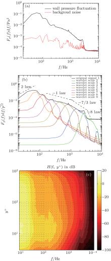
According to , spectrum analysis is applied to p′ and some results are presented in Fig. 7. Figure 7(a) shows the comparison between wall pressure fluctuation and background noise attained by placing the same microphone with the whole accessory outside the wind tunnel at work. It is obvious that the noise interferences from the wind tunnel and external environment are rather small.

Fig. 7.

	Figure Option ViewDownloadNew Window
	Fig. 7. (a) Spectrum curves of p′ and background noise; (b) spectrum curves of p′ and (defined later) in various scales; (c) distribution of transform function H in plane(f, y+ ).

The scaling behavior of the wall pressure spectrum can be seen in Fig. 7(b). These scaling laws link spectral features with different portions of the TBL.^{[19, 44– 49]} The middle frequency region which exhibits an f^{− 1} dependency is associated with the logarithmic region of the TBL. The frequency width of this region is dependent on the Reynolds number. While its upper-bound is nearly independent of Re_θ , the lower-bound has negative correlation with Re_θ . The present data with Re_θ = 2519 show a lower-bound at that is larger than the result of 0.05 with Re_θ = 3386 given by Farabee and Casarella.^[19] The reason is that u_τ increases largely with Re_θ increasing, while f of the lower bound hardly changes. At higher frequencies, the roll-off region is associated with the inner portion of the boundary layer. At frequencies just above the f^{− 1} law region, there is a small region with an f^{− 7/3} slope linked to the buffer layer. Beyond this buffer region, an f^{− 8} slope appears. It is larger than the slope of f^{− 5} attained by Gravante et al.^[44] and Goody.^[47] The larger slope in the roll off region has also been seen in other studies.^{[19, 48, 49]} This may be due to spatial average over the pin-holes. The insufficiently small microphone pinhole size leads to a more rapid roll-off in the case of signal attenuation due to signal averaging; ^[44] it may also be the reason why a small bulge at f = 2.4 kHz appears. The low frequency spectrum just before the f^{− 1} region is associated with the outer portion of the TBL and exhibits a slope of f². Though a relatively low resolution of the Bartlett method in the low frequency range leads to the not-smooth spectrum curve, the detection of f² scaling suggests the ability of our measurement system in a wide frequency-response range.

Although spectral analysis could not reveal all the secrets, it does provide another perspective for this relationship between u′ and p′ . We define a dimensionless transfer function, H, as follows:^[50]

It represents the system with p′ as an input signal and u′ at different values of y⁺ as an output signal. As figure 7(c) shows, the buffer layer has a response in greater intensity and a wider frequency range than in other portions in the TBL. At about , f ≈ 10 Hz, a maximum exists in the (f, y⁺ ) plane. Even at , i.e., f ≈ 300 Hz, the response in the buffer layer is nearly one order of magnitude larger than those in the viscous sub-layer and the log law region. The relation between u′ in the buffer layer and p′ exists in a wide frequency range. This gives us a basis to simplify the control strategy, from opposition control which needs velocity fluctuation information at y⁺ < 20 for practical implementation, to sub-optimal control which only needs wall pressure information.^{[10– 15]} It also offers us a frequency range, , for relatively efficient wall control of the TBL.

In order to analyze the multi-scale nature and detect the most energetic quasi-periodic components, wavelet decomposition is accomplished by projecting signals p′ and u′ on the basis of compact support functions which are localized both in the time and frequency domains.^{[51– 55]} The orthonormal discrete wavelet transform is performed with a db5 wavelet by a fast-wavelet-transform algorithm, i.e., Mallat’ s pyramidal algorithm.^[54] For this fast algorithm, multi-resolution wavelet decomposition and reconstruction can be conducted at the relatively small expense of time and memory. Finally, the reconstructed signals and are attained in terms of time t and resolution scale n.

Localized events missed by the Fourier decomposition are correctly detected by the wavelet transform over the time-frequency domain. Figure 8(a) shows the time evolutions of structures in different scales contained in signal p′ . This is the so-called multi-fractal. These structures are obviously quasi-periodic, the same as the coherent eddy structures in the TBL. The period becomes longer with scale index n increasing. The ribbons in red and blue represent the interactions of wall pressure coherent structures. Ribbons with a positive slope show that small structures merge into a larger one, while ribbons with a negative slope represent the split of a relatively large structure. This cascade phenomenon and its reverse process, from the viewpoint of energy transfer, seem to be more obvious above scale index 4. In Fig. 8(b), the auto-correlation of also provides some information about the period and intensity of the pressure coherent structure. The structures in the region of scale index 8 own the most portion of pressure fluctuation energy, and the structures in the region below the scale index 4 exhibit weak coherence.

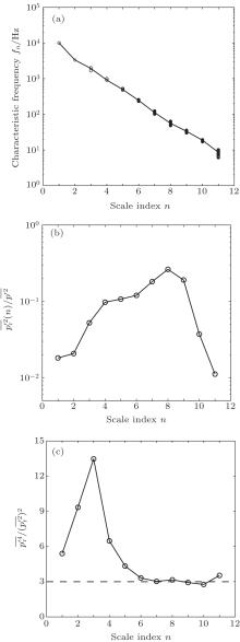
There exists an obvious relationship that n is linearly varying with logarithmic f_n as seen in Fig. 9(a). The fitting result of the scatters is well consistent with the theoretical formula,

Here, A = − log 2 describes the dyadic property of the wavelet transform and B = log f_samp shows its dependence on signal sampling frequency f_samp.

Fig. 8.

	Figure Option ViewDownloadNew Window
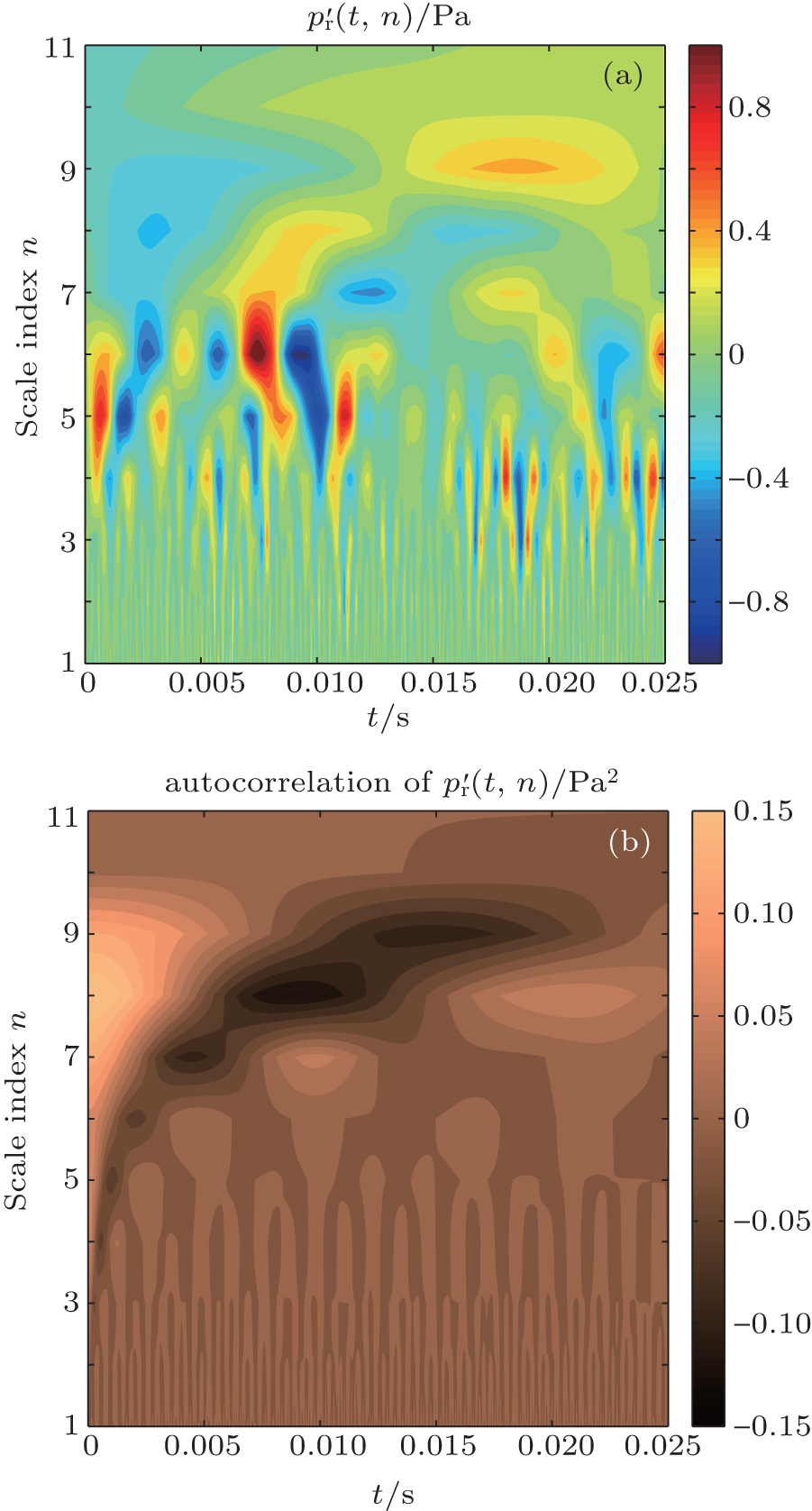	Fig. 8. (a) Reconstructed wall pressure fluctuation (b) auto-correlation of .

Fig. 9.

	Figure Option ViewDownloadNew Window
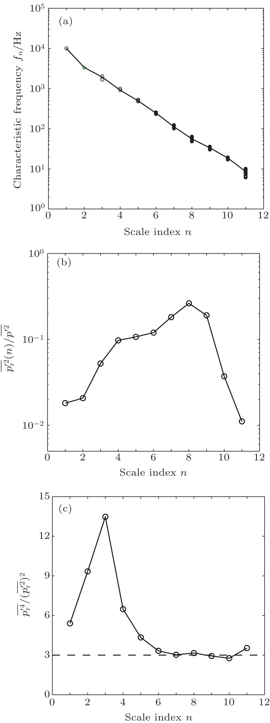	Fig. 9. Statistic results of (a) relation between fn and n; distributions of (b) and (c) in scale n.

Figure 9(b) provides information about the relative energy distribution of p′ among these 11 scale indices. is the time average of the square of shows that the most energetic quasi-periodic structures are in the range of scale index 8, corresponding to f₈ ≈ 80 Hz. This conclusion agrees with that from Fig. 7(b) in which the FFTs of are shown. In Fig. 7(b), the curve of each scale index manifests as a prominent peak located at the characteristic frequency f_n, by which the wavelet transform with db5 shows good locality in the frequency domain.

The flatness of , reaches a peak greater than 13 as n = 3n in Fig. 9(c). Finally, the flatness keeps stable at 3 as n ≥ 6. The pressure coherent structures in the range with scale index n < 6 show intermittency, while the ones in a range with scale index n ≥ 6 do not. The strong intermittency in the range with scale index 3, corresponding to f₃ ≈ 1.9 kHz, is associated with the buffer layer characterized by f^{− 7/3} law of the p′ power spectrum curve.

The time-frequency distributions of at y⁺ = 5.2, 15.5, 51.7, and 621 are presented in Fig. 10. The velocity coherent structures in the buffer layer are more intensive and intermittent. Meanwhile, the interaction of structures, such as merge and split, is also strong in this portion.

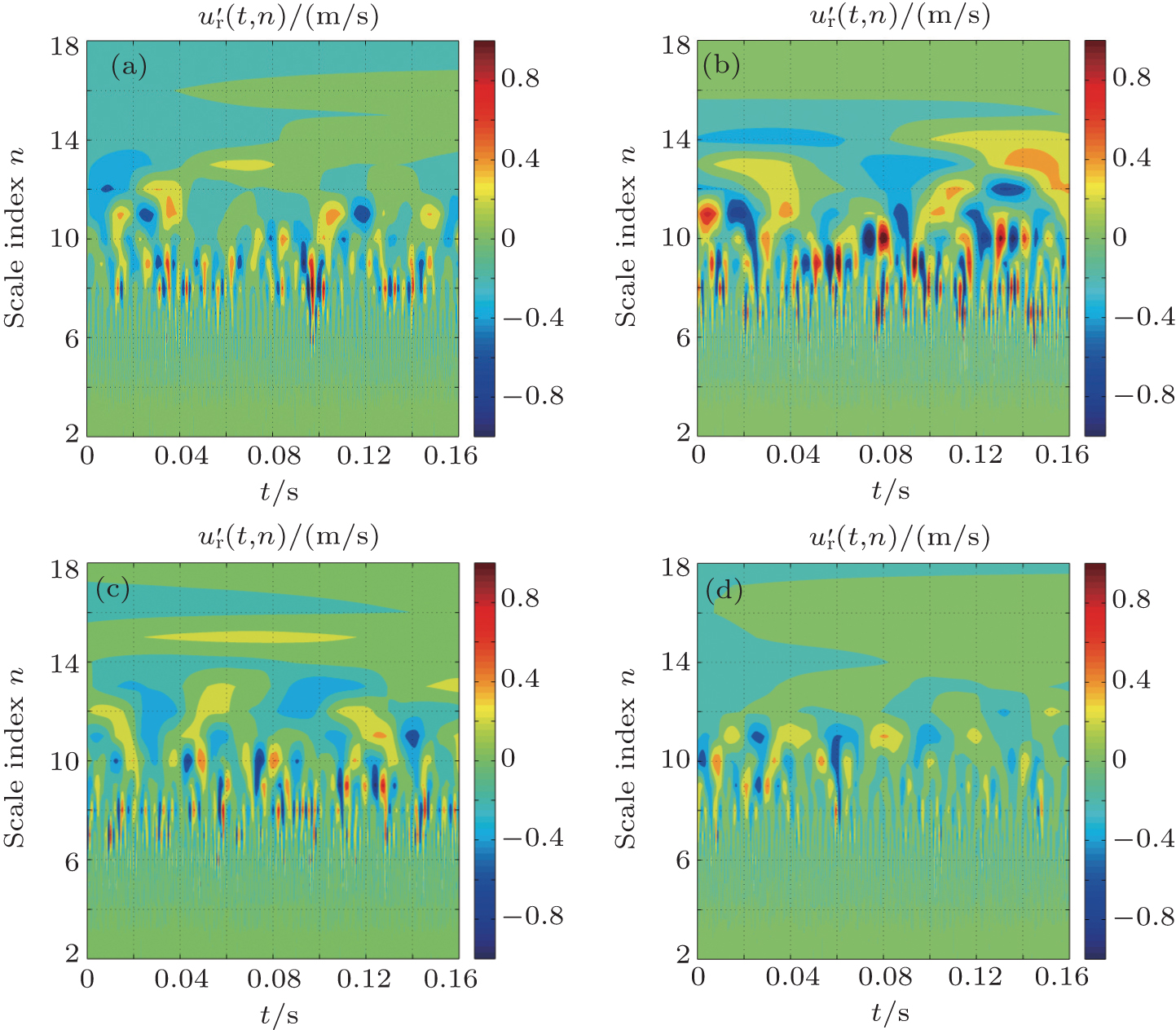Fig. 10.

	Figure Option ViewDownloadNew Window
	Fig. 10. at (a) y+ = 5.2, (b) y+ = 15.5, (c) y+ = 51.7, (d) y+ = 621 in TBL.

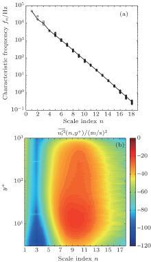
Figure 11(a) shows the relationship between n and f_n for u′ . The linear logarithmic relation still exists due to the intrinsic nature of wavelet transform instead of the physical phenomenon under study. The energy distribution in plane (n, y⁺ ) of is shown in dB (Fig. 11(b)). A complete peak is evident and compared with that in Fig. 6(b), and the maximum of at (n = 9, y⁺ = 14) provides more specific frequency f₉ ≈ 147 Hz for active control.

Fig. 11.

	Figure Option ViewDownloadNew Window
	Fig. 11. Statistic results of (a) relation between fn and n; (b) distribution of in plane (n, y+ ).

For velocity fluctuation measurement near the wall by HWA, the special miniature boundary layer probe is the key device. In addition to the shape and size of probe, the length l⁺ and the ratio l/d of the sensor wire are important parameters. Very simple practical rules show that l⁺ as small as possible and a large enough l/d are appropriate. On the other hand, a high enough sampling frequency is necessary for detecting the small scale velocity components. The mean velocity and turbulent intensity profiles, as well as the analyses about Kolmogorov dissipation scale η , Taylor differential scale λ , and integral scale L, prove that our measurement for u′ is valid to study the multi-scale nature of a fully developed TBL in an equilibrium state. PDF, skewness, and Kurtosis results show the statistic properties of the four portions in the TBL, i.e., the viscous sub-layer, buffer layer, log law region, and wake region. The buffer layer with strong intensity and intermittency is especially attractive for active control.

The microphone placed in the pin-hole mechanism has a relatively high spatial resolution for the wall pressure fluctuation measurement beneath the TBL. Dimensionless coefficient is 3.06 for Re_τ = 996Re_τ p′ . In addition, the comparison between wall pressure and background noise in the frequency domain indicates that the noise interference from the wind tunnel and external environment is rather small and our measurement could detect the wall pressure fluctuations with a certain precision.

Both u′ and p′ signals manifest as the exponent scaling laws in the frequency domain. The former is associated with the energy cascade and the latter links spectral features with different portions of the TBL. The power spectrum and dissipation spectrum of u′ show the evident inner peaks Re_τ . By treating TBL flow as a system with p′ as input and u′ as output, the transfer function reveals the close relationship between u′ in the buffer layer and p′ in a wide frequency domain.

Compared with the Fourier transform, the wavelet transform shows its good locality in the frequency domain. As a time-frequency analysis method, the wavelet transform reveals the intermittent multi-fractal structures contained in both u′ and p′ signals. The wavelet scale index n varies linearly with logarithmic characteristic frequency f_n. The scale which owns most of the intermittency of p′ is associated with the coherent structure in the buffer layer characterized by f^{− 7/3} scaling law. It is worth noting that the maximum of at (n = 9, y⁺ = 14) provides a specific frequency f₉ ≈ 147 Hz for wall actuating active control with Re_τ = 996.