


Stability analysis for flow past a cylinder via lattice Boltzmann method and dynamic mode decomposition
[Zhang Weia) , Wang Yongb)†  , Qian Yue-Hong
b) ]
, Qian Yue-Hong|
|


†Corresponding author. E-mail: ywangcam@gmail.com, yongw2@uci.edu
A combination of the lattice Boltzmann method and the most recently developed dynamic mode decomposition is proposed for stability analysis. The simulations are performed on a graphical processing unit. Stability of the flow past a cylinder at supercritical state, Re = 50, is studied by the combination for both the exponential growing and the limit cycle regimes. The Ritz values, energy spectrum, and modes for both regimes are presented and compared with the Koopman eigenvalues. For harmonic-like periodic flow in the limit cycle, global analysis from the combination gives the same results as those from the Koopman analysis. For transient flow as in the exponential growth regime, the combination can provide more reasonable results. It is demonstrated that the combination of the lattice Boltzmann method and the dynamic mode decomposition is powerful and can be used for stability analysis for more complex flows.
Since its inception two decades ago, the lattice Boltzmann method (LBM) has emerged as an alternative and promising numerical approach for computational fluid dynamics (CFD).[1– 6] The LBM is based on the kinetic theory of gases and used to resolve the macroscopic fluid dynamics.[2] Different from the conventional incompressible Navier– Stokes (NS) solver, the LBM does not solve the Poisson equation for pressure, which involves global data communication. Instead data communication is always local and the pressure is obtained through an equation of state in the LBM. In other words, the LBM is readily parallelizable. Moreover, the mesh generation for the LBM is much faster than that for the conventional methods of NS equations, such as the finite difference method (FDM), the finite element method (FEM), and so on. That means the LBM can easily model fluid flows with complex geometries and boundary conditions. Accordingly, the LBM has been widely adapted in fields such as aerodynamics[7] and biomechanics[8] with complex flows, including flow separation, turbulence, and other transient flows of critical situations.
For simulating such unstable flows, the results are always very sensitive to the numerical methods, in which the solvers’ dissipation and dispersion relation plays a very important role. Meanwhile, stability analysis is a very important tool for analyzing such flows. For stability analysis, the technology of linearized NS equations and then shifting to the eigenvalue problem is still a major method. One can easily extend the nonlinear NS solver to a linear analysis solver in the conventional method.[9] To the best of the authors’ knowledge, there are only several published papers about stability analysis for fluid flows via the LBM. To perform Von Neumann stability analysis from the linearized LB equation[10, 11] is a way for stability analysis in the LBM. But as shown in these references, the way in the LBM is not as straightforward as that in conventional methods. One more challenge in the LBM is to get the so-called base flow for stability analysis as there is no existing base flow solver for complex flow problems.[12] As a result, only simple cases whose base flow can be expressed analytically were studied in the references.
Most recently, dynamic mode decomposition (DMD), which is a linear decomposition technique developed for extracting dynamic modes that can approximate the underlying nonlinear dynamics, was shown by Schmid.[13] This technique is linked to the Koopman analysis, which was recently applied to an analysis of fluid mechanics problems.[14] The DMD can be applied for analysis of data from both experimental and numerical results.[15] Comparing with convention decomposition techniques such as discrete Fourier transform (DFT) or proper orthogonal decomposition (POD), as shown in Ref. [16], the DMD can get growth rates and frequencies associated with each mode. Hence the DMD can be interpreted as generalization of global stability. Furthermore, from a numerical point of view, one can use data generated by the solver for stability analysis directly, which means that no extra programming is needed. These features lead the DMD to be a very powerful tool for stability analysis.
The authors also noticed that Brownlee et al. in Ref. [11] predicted an unstable behavior for the flow past a cylinder at subcritical Reynolds number, Re, via the LBM. This leads us to being interested in the performance of the LBM to predict transient flow at such a critical situation. In the present work, stability analysis is carried out for flow past a cylinder at Re = 50, which is slightly larger than the critical value of the first kind of instability of flow separation, by the LBM simulation and using the results as snapshots for the DMD to perform stability analysis to get physical instability. The other reason to select this test case is that present results can be compared with those in a recently published work performed by the Koopman analysis[14] for the same Re number. To attain decent resolution, we did systematically mesh a refinement study in advance. A mesh with about 2× 10⁷ lattices was selected for productive simulations. Such mesh is at the DNS level. It is demonstrated that with such a mesh resolution, one can predict the flows around the critical Re number and get accurate flow fields. Due to such a fine resolution, simulations were performed on a graphical processing unit (GPU). The high-end GPU works with lower frequency than the central processing unit (CPU), but has access to fast memory and contains many more cores on a single device. This means a single GPU can replace a small cluster while being cheaper and using less power.[17] Moreover, as we mentioned before, the LBM is readily parallelizable and especially suitable for running on a GPU machine.[18] That is to say we can gain newly computing power with the LBM to get a fine enough resolution and a reasonable solution. To use such DNS level solutions from fine resolution simulation as snapshots to carry out DMD analysis means that they can be used for physical instability analysis while avoiding complex mathematical work. Moreover, to the best of the authors’ knowledge, there is no published paper about stability analysis with the combination of the LBM and the DMD. Such a combination has the advantages of both methods as mentioned above.
The remainder of this paper is organized as follows. Formulations of the LBM and the DMD are given in Section 2. Details of the physical model and performance test for the code are presented in Section 3. Results for the exponential growing regime and the limit cycle regime are given and analyzed in Section 4. The conclusions are summarized in Section 5.
In this section, we will give a brief summary of the LBM and the DMD.
The main dependent variable of the LBM is the fluid particle density distribution function, f, whose transport is governed by the lattice Boltzmann equation


where, α is the directional index of the discrete velocity vector eα , x is the position of the fluid particle, t is the time, dt is the time step, and τ is the non-dimensional relaxation time. fα and 
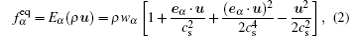
which is derived from the Maxwellian distribution function. The weighting functions wα are determined by satisfying necessary conditions of isotropy of the fourth-order tensor of velocities and Galilean invariance.[1]
The macroscopic (continuum) fluid properties such as density ρ , velocity u, and pressure p are functions of fα according to

The relaxation time τ is a function of the fluid density ρ , the kinematic viscosity ν , the sound speed cs, and the time step dt, according to 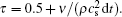
The algorithm of the DMD used here is from Ref. [13]. A brief description is given in the following part. First the data, which are produced by the LBM simulation and separated in time by a constant step △ ts, is represented in the form of a snapshot sequence and given by a matrix 

Therefore eigenvalues of A give the growth rate and frequency of each mode. Snapshots become linearly independent with sufficient number. This can be written in the vector form as

where r is the residual. By using singular value decomposition (SVD), S can be solved with minimizing residual r. So the Ritz values of S are used to approximate those of A, and the Ritz vectors of S are used to construct the modes as shown in Ref. [13].
In this work, flows around a cylinder especially at Reynolds number, Re= 50, were carefully studied, while other simulations for Re ∈ [40, 160] were also carried out for validation. Therein, Re is calculated with the inlet velocity U, diameter of the cylinder D, and the viscosity ν according to Re = U × D/ν . A rectangle computation domain with size Lx × Ly = 61D × 50D was used. The cylinder was placed in the domain with its center located at x = 16D and y = 25D. The wall of the cylinder was considered to be non-slip and treated with the bounce-back scheme. A slip boundary condition was imposed at the top and bottom boundaries. A constant velocity U was prescribed at the inlet (x = 0) boundary. A full-developed boundary was applied at the outlet boundary (x = Lx). The GPU-based LBM solver used here is the open source code, Sailfish.[20]
As mentioned before, a GPU works with lower frequency than a CPU, but has access to fast memory and contains many more cores on a single device. In the present study, simulations were performed on from single to four Tesla K20M cards. There are 13 processors on every GPU card, and each processor has 196 cores. In other words, there are 2496 cores on each Tesla K20M card.
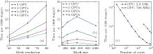
The performance of the code was tested with difference mesh size, block size, and number of GPU cards before productive simulations, and is presented in Fig. 1. In particular, the performance versus the number of lattices per cylinder diameter, ND = 40, 60, and 80 are given in Fig. 1(a). The clock time used for every 1000 time steps is given for comparison. The lower clock time used the better numerical performance it has. It can be seen that with the increase of ND, more and more clock times are needed. On the other hand, with the increase of the number of GPU cards, lower clock time is needed. ND = 80 lattices are chosen in the following simulations.
 | Fig. 1. Performance of the code. (a) Performance versus mesh resolution, (b) performance versus block size, and (c) scalability study. |
Every LBM node in the code is processed in a separate GPU thread, and these threads are grouped into one dimensional blocks for data exchange.[20] The block size is thus another tunable parameter that has an effect on the performance, as shown in Fig. 1(b). For a simple case, the larger number block size would result in better performance; for complex cases, such a relationship is dependent on the cases. In the present study, the best performance can be found when the block size is 64.
The performance of the code on the GPU is also compared with that on the CPU with another open source code of LBM, Palabos, [21] for a mesh with ND = 80. The later run on a supercomputer Blue Waters, [22] which has 22640 Cray XE6 nodes (each containing 2 AMD Interlagos processors and 16 cores per processor) and 4224 Cray XK7 nodes (each containing one AMD Interlagos processor). As shown in Fig. 1(c), up to 10192 GPU cores (or 52 processors, 4 Tesla K20M cards) and 8192 CPU cores (or 512 processors) were used, respectively. Both codes have good scalability on corresponding computing platforms. Moreover, the performance of 10192 GPU cores is similar to that of about 800 CPU cores. Considering the difference of clock speeds (2.3 GHz for CPU and 706 MHz for GPU), such performance is acceptable. Anyway, one can see that the performance of several GPU cards is comparable with that of a traditional cluster or even supercomputer.
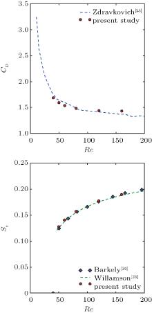
First of all, the resulting drag coefficient, CD(= FD/(0.5× ρ U2)), and Strouhal number, St(= fD/U), for different Re numbers in the range of [40, 160] are compared with those from references. It can be seen from Fig. 2(a) that the obtained results of CD agree well with those from Zdravkovich’ s simulation.[23] For St, the dash line in Fig. 2(b) is from the three-term fit by Willason and Brown, [24] where St is given by

for Re ∈ [50, 200]. Again, the obtained St via the LBM agrees well with the regression formula and the data from Ref. [25] via the high order method. Especially for cases Re = 40 and Re = 50, which are around the bifurcation point Rec = 46.6, the current solver can fully capture the different flow regime.
 | Fig. 2. Comparison of predicted drag coefficient and Strouhal number with the results in references: (a) CD versus Re, (b) St versus Re. |
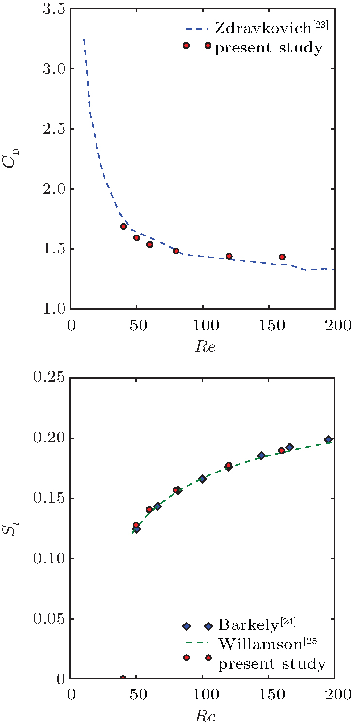
In this subsection, we focus on the flow at Re = 50. The time history of lift force coefficient (CL) on the cylinder is shown in Fig. 3. As in Refs. [14] and [16], different time scales can be identified in different time intervals. In Fig. 3(a), there is an exponential growing of CL in time interval [400, 800]. Within this interval, amplification, A, can be studied by means of Stuart– Landau amplitude equation[14]

where σ r in the first part of the right-hand side of Eq. (7) is a linear growth rate, and equal to 0.012 in the present study as shown in Fig. 3(b). Besides, in the interval [1200, 1500] the flow ultimately approaches the saturated limit cycle. In the following part, the DMD analysis is carried out for these two different intervals, where the snapshots are from the LBM simulation with sampling interval Δ ts = 0.3333 s.
 | Fig. 3. Time history of lift coefficient (a) CL and (b) | CL| . |
The Ritz values and energy spectrum of a data set within time interval [1200, 1500] are shown in Figs. 4(a) and 4(c). The Ritz values of the three most energetic ones, corresponding to modes 0 to 2, and even higher order transient modes lies on the unit circle in Fig. 4(a), indicating that the corresponding modes are neither growth nor decay. They are partitioned equally with angle θ relative to St in the way St = arctan(θ )/2π Δ ts. Such a phenomenon was also found in Refs. [14] and [16]. It can be interpolated that the flow’ s periodic orbit exhibits harmonic-like behavior. The results from the DMD are also compared with the Koopman eigenvalues of the NS equations from Ref. [14] in Fig. 4(b). This is accomplished by the logarithmic mapping of the eigenvalues according to μ = log(λ )/Δ ts. The values of μ for modes 0 to 2 and their complex conjugate are at axis y = 0, and the same as those from the Koopman analysis. Moreover, the ones for modes 3 to 5 can be observed in Fig. 4(b), while they cannot be seen clearly due to a visualization reason in Fig. 4(a). Horizontally, they are distributed in a similar way to the corresponding Koopman eigenvalues in Fig. 4(b).
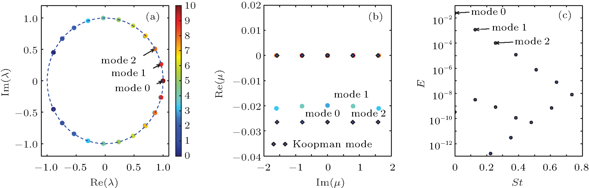 | Fig. 4. Ritz values computed from the DMD on the LBM results for flow in time interval [1200, 1500]. (a) Ritz values, (b) Ritz values versus the Koopman eigenvalues, (c) energy spectrum. |
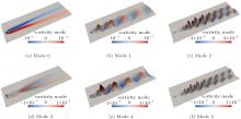
All modes marked in Fig. 4 are shown in Fig. 5 in vorticity. Modes 0 to 5 correspond to the mean flow, global mode, second harmonic mode, shift mode, transient global mode, and transient second harmonic mode respectively in the Koopman analysis. Vortex structures in modes 0, 1, 3, and 4 are symmetric, which correspond to large-scale convection of fluid structures in the wake, while modes 2 and 5 are anti-symmetric and correspond to the alternative shedding of the Von Karman vortex street.
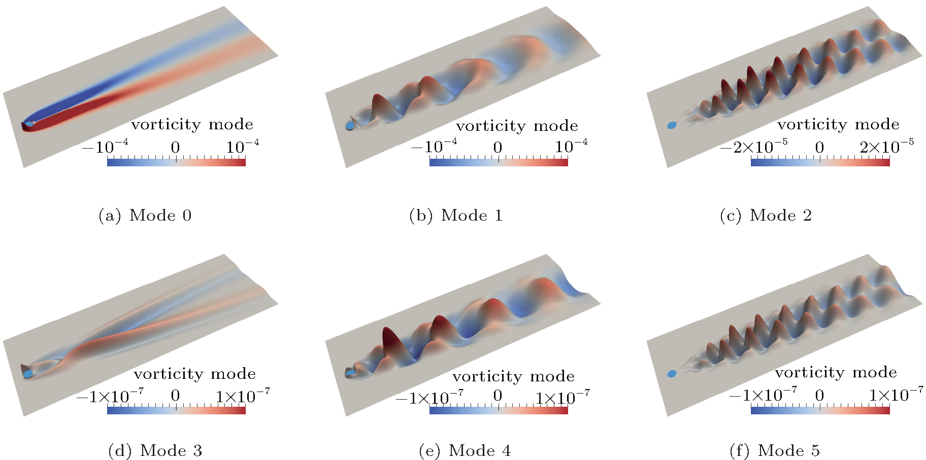 | Fig. 5. Several main modes for flow in time interval [1200, 1500]. Modes 0– 5 correspond to panels (a)– (f). |
The DMD results of the exponential growing regime in interval [400, 800] are shown in Figs. 6 and 7. It can be seen from Fig. 6(a) that all the Ritz values lie outside the unit cycle. So in Fig. 6(b), all the corresponding values are positive. This is different from the results in Ref. [14], in which Bagheri collected snapshots in the whole transit range including the limit cycle as well as the nonlinear growing part and stated that the results are sensitive to the snapshots in their paper and their collection is not reasonable. It can be interpolated, with the data set we selected here, that an almost linear dynamics is observed and so the growth rate should be positive. We also noticed that even if there are double the number of snapshots, the DMD results are the same. It can be seen in Fig. 6(b), that the growth rate of the most energetic growing mode, mode 1, is 0.012. This value is the same as the σ r of the lift coefficient within the exponential interval. The growth rate of mode 2 is twice that of mode 1. Besides in Fig. 6(c), the energy spectrum is not as regular as in Fig. 4(c). This is due to the higher order non-linearity, which needs a cluster of complex modes to describe it.
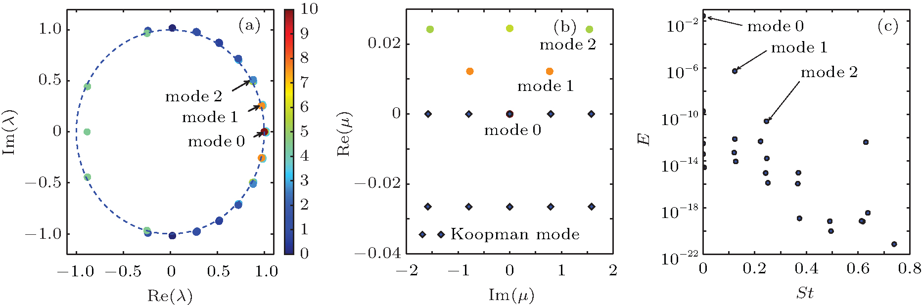 | Fig. 6. Ritz values computed from the DMD on the LBM results for flow in time interval [400, 800]. Panel (a) for Ritz values, (b) Ritz values versus the Koopman eigenvalues, (c) energy spectrum. |
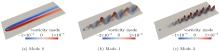
Mode 0, in Fig. 7(a), has a longer tail than the equivalent mode in the limit cycle in Fig. 5(a). This is because mode 0 is of the base flow, where the perturbation grows, rather than the mean flow of a fully developed flow past a cylinder. Mode 1 has a symmetrical vortex structure as shown in Fig. 7(b), like the equivalent mode in the limit cycle in Fig. 5. It is similar to the results of the linear stability analysis in Refs. [26] and [27], in which the leading eigen-mode has the same symmetrical vortex structure. Since mode 1 has the same value of growth rate as that of CL, this means within this interval the growing of CL amplitude is dominated by large-scale convection of fluid structures in the wake. Mode 2 has an anti-symmetrical vortex structure as shown in Fig. 7(c). The amplitude of the vorticity in the vortex center in this mode keeps growing downstream, this indicates that the alternative shedding of the Von Karman vortex street starts from a convective instability.
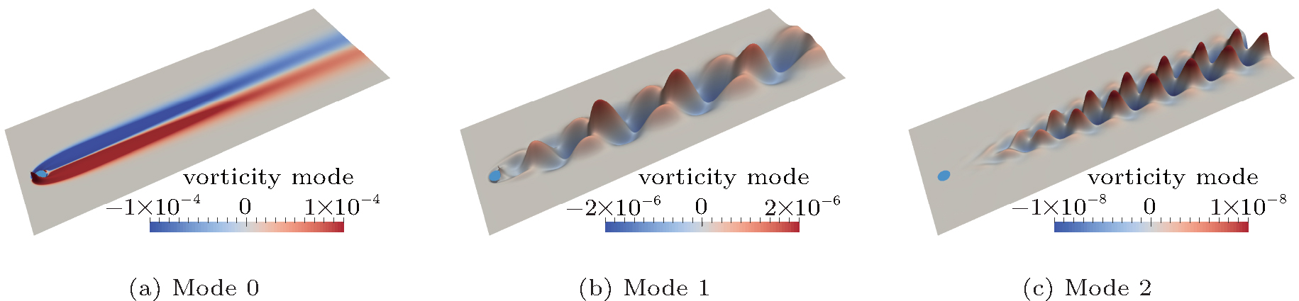 | Fig. 7. Several main modes for flow in time interval [400, 800]. Panels (a)– (c) correspond to modes 0– 2. |
In this study, stability analysis for the flow past a cylinder was performed with the LBM and the DMD. The simulation was carried out on GPU machines, and its performance was tested first. It is demonstrated that the performance of several GPU cards is comparable with that of a conventional cluster or even a supercomputer with CPU.
The flows at different Re numbers in the range of [40, 160] were simulated for validation. The obtained drag coefficient, CD, and Strouhal number, St, agree well with those in the references with other numerical methods. Specially, global stability of the flow at supercritical state, Re = 50, was studied by the combination of the LBM and the DMD for both the exponential growing and limit cycle regimes. The Ritz values for both regimes are presented and compared with the Koopman eigenvalues. Several main modes are given and discussed. Within this work, we showed the following facts.
(i) With the help of the DMD, we can use the LBM to carry out global stability analysis numerically and get the transient flow behavior like global Strouhal number St, transient growth rate σ r as well as the modes for certain regimes.
(ii) For harmonic-like periodic flow as in the limit cycle, global analysis from the combination of the DMD and the LBM gives the same results as those from the Koopman analysis.
(iii) For transient flow as in the exponential growth regime, the combination of the LBM with the DMD can provide more reasonable results comparing with the Koopman analysis, since the latter can only provide a bounded solution.
In summary, it can be concluded that the combination of the LBM and the DMD is powerful and can be used for stability analysis for more complex flows.
| 1 |
|
| 2 |
|
| 3 |
|
| 4 |
|
| 5 |
|
| 6 |
|
| 7 |
|
| 8 |
|
| 9 |
|
| 10 |
|
| 11 |
|
| 12 |
|
| 13 |
|
| 14 |
|
| 15 |
|
| 16 |
|
| 17 |
|
| 18 |
|
| 19 |
|
| 20 |
|
| 21 |
|
| 22 |
|
| 23 |
|
| 24 |
|
| 25 |
|
| 26 |
|
| 27 |
|