


A scheme for two-photon lasing with two coupled flux qubits in circuit quantum electrodynamics*
[Huang Wena), b) , Zou Xu-Boa), b)†  , Guo Guang-Can
a), b) ]
, Guo Guang-Can|
|


†Corresponding author. E-mail: xbz@ustc.edu.cn
*Project supported by the National Fundamental Research Program of China (Grant No. 2011cba00200), the National Natural Science Foundation of China (Grant No. 11274295), and the Doctor Foundation of Education Ministry of China (Grant No. 20113402110059).
We theoretically study the system of a superconducting transmission line resonator coupled to two interacting superconducting flux qubits. It is shown that under certain conditions the resonator mode can be tuned to two-photon resonance between the ground state and the highest excited state while the middle excited states are far-off resonance. Furthermore, we study the steady-state properties of the flux qubits and resonator, such as the photon statistics, the spectrum and squeezing of the resonator, and demonstrate that two-photon laser can be implemented with current experimental technology.
Two-photon laser, which is on the basis of the stimulated emission processes of photon pairs, has drawn continued attention since the original concept in the 1960s[1– 5] and has found significant applications in quantum information[6, 7] and quantum telecommunication.[8] Experimentally, two-photon laser has been realized in the atomic system.[9] Further theoretical works discuss the possibilities of two-photon laser in the semiconductor, [10– 14] and two-photon emission in semiconductor systems has been experimentally demonstrated.[15– 20]
In the past decades, superconducting qubits acting as artificial two-level atoms have been used to investigate many basic quantum effects such as Rabi oscillations and Ramsey fringes.[21– 23] Two coupled qubits can be considered as a multi-level atom, the coupling of qubits is controllable[24, 25] and the spectroscopy measurements on two coupled flux qubits has been performed.[26, 27] Moreover, a new field called circuit quantum electrodynamics (QED) has been opened up by coupling superconducting qubits to electromagnetic resonators. It is analogue of ‘ cavity QED’ with superconducting qubits behaving as atoms and an electromagnetic resonator replacing the cavity. In comparison with cavity QED, circuit QED offers the controllability inherent to solid-state circuits and strong coupling between the qubits and the resonator modes. So far, the resonators have been applied in quantum information processing such as to prepare and read out the qubit state[28– 32] or to perform single- and two-qubit gates.[33– 37]
Recently, several experiments have been performed to realize single photon laser.[38, 39] In particular, the single photon lasing action was demonstrated based on a single charge qubit coupled capacitively to a microstripline resonator, [38] and the population inversion was realized incoherently by single-electron tunneling events. In Ref. [39], a driven flux qubit was also used to realize single photon lasing by coupling to a low-frequency LC resonator.
In this paper, we demonstrate a two-photon lasing scheme by coupling two superconducting flux qubits to a superconducting transmission line resonator. It is shown that due to the interaction of the two qubits, the resonator mode can be tuned to two-photon resonance between the ground state and the highest state while the middle states are far-off resonance. Moreover, we consider the dissipation and the incoherent pumping, study the steady-state properties of the system, such as the photon statistics, the spectrum, and squeezing of the resonator, and demonstrate that such a system may be appropriate for two-photon lasing.
The paper is organized as follows. In Section 2, we introduce the model of a resonator coupled to two interacting flux qubits. In Section 3, an effective Hamiltonian is given for two-photon resonant interaction. We also consider the coherent dynamics for illuminating how to enhance the two-photon processes. In Section 4, we consider the incoherent pumping and the dissipation, and study the steady-state properties of the system, such as the photon statistics, the spectrum, and squeezing of the resonator. Finally, a conclusion is given in Section 5.
The system we study is a single mode quantum resonator coupled to two qubits (see Fig. 1(a)). Although our analysis bears a general character, superconducting flux qubits[40] are considered for concreteness. We describe the two flux qubits at first. Suppose the two superconducting rings with three Josephson junctions are respectively controlled by constant magnetic fluxes Φ i (i = 1, 2) and the coupling between the two qubits is determined by an Ising-type (inductive coupling) term 

where Δ i is the tunnelling amplitude, and 

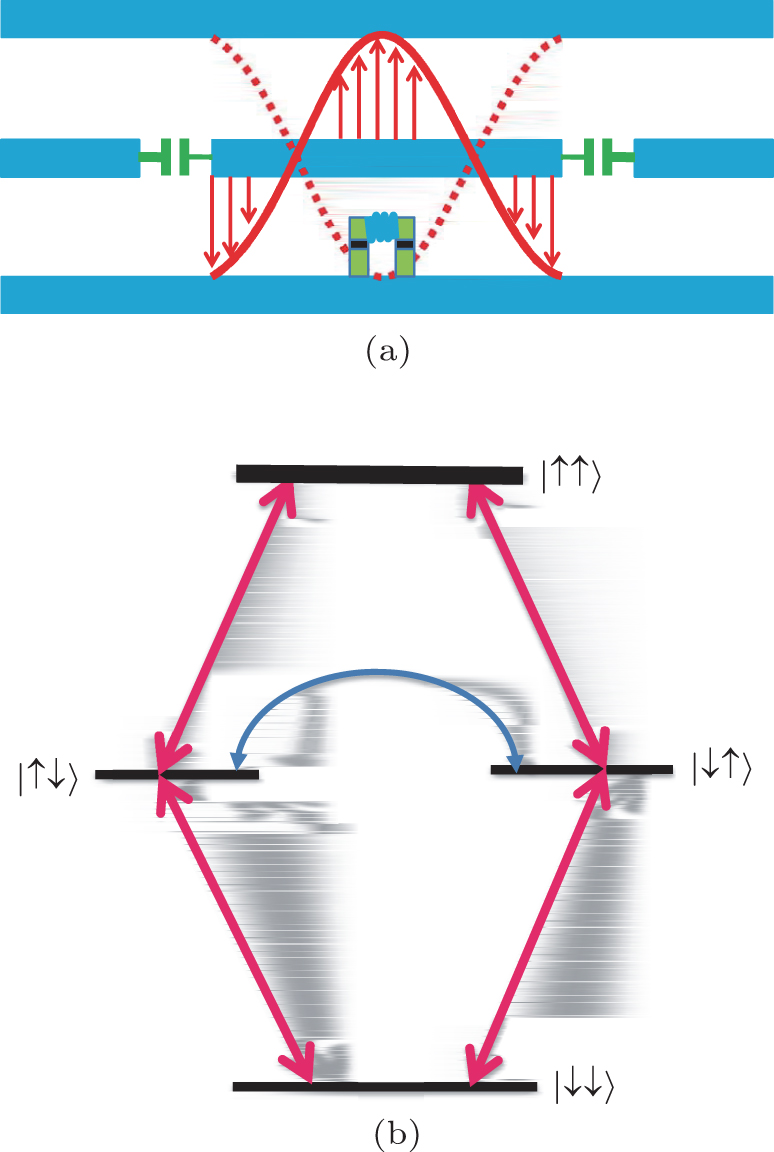 | Fig. 1. (a) Schematic diagram for a coupled system of two flux qubits and a transmission line resonator. The two qubits are coupled inductively. (b) The level diagram for the two qubits. The red double arrows show the couplings with the resonator, and the dark blue double arrow shows the coupling between the two qubits. |
Then we consider the coupling of the two flux qubits to the one-dimensional transmission line resonator, although it supports various modes, we consider one mode only, so the Hamiltonian is

where we set ħ = 1, ω a is the frequency of the resonator, a† and a are the photon creation and annihilation operators respectively, and gi is the coupling strength between the i-th qubit and the resonator. We bias the superconducting rings at the flux degeneracy point (fi = 0) and suppose the two qubits are identical, Δ 1 = Δ 2 = Δ , g1 = g2 = g. After transformations to the eigenbasis of each qubit and a rotating wave approximation, the Hamiltonian reduces to

The Pauli matrices act on the single-qubit eigenstates 
Since the dynamics of the system is strongly affected by the incoherent processes which contain the dissipation and the incoherent pumping, we now consider them using the density matrix approach. The master equation for the reduced density matrix of the qubits and the resonator reads

where we have used the Liouville operators 


and
where κ is the strength of the resonator damping, γ i is the relaxation rate of each qubit and pi characterizes the incoherent pumping strength. In what follows we assume that the two identical qubits suffer the same relaxation rate and pumping rate, that is γ 1 = γ 2 = γ , p1 = p2 = p. Equation (5) represents the loss of the resonator and equation (6) contains the qubits dissipation and the pumping processes. Here the qubits system is continuously pumped by an incoherent process, and the population inversion can be realized due to the competition between coherent coupling, incoherent pumping, and dissipation, which we will show later.
For the sake of showing the two-photon processes intuitively and analyzing the significance of the parameters for two-photon processes exceeding one-photon processes, we will derive the effective Hamiltonian using some approximations and then concentrate on the coherent dynamics of the qubits coupled with the resonator, discarding any kind of dissipation temporarily. Firstly we represent the Hamiltonian (3) using the single qubit eigenstates
where the state vectors for the two-qubit system {| ↓ ↓ 〉 , | ↓ ↑ 〉 , | ↑ ↓ 〉 , | ↑ ↑ 〉 | }are composed from the single-qubit states: | ↓ ↓ 〉 = | ↓ 1〉 | ↓ 2〉 , etc. By introducing the following states 


It shows that the state | − 〉 has no coupling with the resonator. By applying the Schrieffer– Wolff transformation[43] and the effective Hamiltonian theory[44] we obtain a Hamiltonian for the reduced Hilbert space of the qubits states{ | ↓ ↓ 〉 , | ↑ ↑ 〉 } and for the resonator-mode states at two-photon resonance between ground state | ↓ ↓ 〉 and the highest excited state | ↑ ↑ 〉 (δ = 2Δ − 2ω a = 0)
The last term exhibits the two-photon processes, and the effective Hamiltonian (9) is obtained by assuming J ≫ g, which can be easily satisfied in experiment. At the same time, the coupling constant g between the qubits and the resonator should not be too small for guaranteeing that the two-photon processes are not so weak. Therefore, in the following we will adopt the parameter g/2π = 0.1 GHz.
In Fig. 2 we show the populations of the qubits states as a function of the time numerically to illuminate the importance of coupling constant J between two superconducting qubits for distinguishing the two-photon processes from one-photon processes. We plot the curves by solving numerically Eq. (4), setting the incoherent terms to zero and assuming that the system is initially in state | ↓ ↓ , 2〉 which indicates that the qubits are in the ground state and there are two photons in the resonator. The upper row corresponds to J = 3.8 while the bottom row J = 0. In Fig. 2(a) the superconducting transmission line resonator is two-photon resonant with the ground state | ↓ ↓ 〉 and the highest state | ↑ ↑ 〉 transition, and it shows the coherent two-photon exchanges between | ↓ ↓ , n〉 and | ↑ ↑ , n − 2〉 with considerable amplitude. When the resonator frequency ω a is far-off resonance from any transition, the population of the initial state is almost unit at all times as shown in Fig. 2(b) and Fig. 2(e). In Fig. 2(c) the resonator frequency is resonant with the transition frequency between | ↑ ↑ 〉 and | + 〉 , and we observe the single-photon Rabi oscillations. When J equals zero, one-photon resonance and two-photon resonance happen at the same time as shown in Fig. 2(d), and both of them are quite strong.
 | Fig. 2. Populations of the qubits states Pξ vary as time by setting the incoherent terms to zero, initially in state | ↓ ↓ , 2〉 . In panels (a)– (c) the coupling constant J = 3.8 (2π GHz) and the two-photon detuning (a) δ = 0, (b) δ = 0.1Δ , (c) δ = J. In panels (d)– (e) the coupling constant J = 0 and the two-photon detuning (d) δ = 0, (e) δ = 0.1Δ . The curves correspond to P| ↓ ↓ 〉 (blue solid lines), P| + 〉 + P| − 〉 (red dotted lines), and P| ↑ ↑ 〉 (green dashed lines). The other parameters are Δ 1 = Δ 2 = 15.8, g = 0.1 (all in units of 2π GHz) in all the five plots. |
In the previous section, we discussed the two-photon resonance in absence of pumping and dissipation, but they play a significant role in the dynamics of the system, so the incoherent processes including the decay of the system and the pumping by continuously external incoherent field will be added in this section. We study the steady state populations, the photon statistics, the spectrum of the resonator output, and the squeeze property by solving the master equation (4) numerically.
The steady state means that the density matrix of the system does not vary with time, in other words, the master equation (4) equals zero. We solve the equation by reasonably cutting down the number of photons in the resonator. The population of the state | j〉 (j = ↓ ↓ , + , − , ↑ ↑ ) is denoted by Pj = 〈 j| ρ | j〉 , and it is certified that P| + 〉 = P| − 〉 . They are significantly decided by the competition between the strong coherent coupling to the resonator mode and the incoherent processes.
We show the steady-state populations as a function of the two-photon detuning δ in Fig. 3, where δ = ± 3.8 correspond to one-photon resonances and δ = 0 corresponds to two-photon resonances. The pumping rate is increasing from panel (a) to panel (d), and we can obviously distinguish the two-photon processes from the one-photon processes. At δ ∼ 3.8, where the | ↑ ↑ 〉 ↔ | + 〉 transition arrives resonantly, the ground state | ↓ ↓ 〉 remains almost empty while the middle state | + 〉 occupation increases obviously due to the depletion of the upper state population. However, at δ ∼ − 3.8 when the | + 〉 ↔ | ↓ ↓ 〉 transition arrives resonantly, the populations of the states suffer few changes, indicating that photon emission between these two states is weak. In addition, at two-photon resonance (δ = 0) we observe a prominent increase of the ground state population while very small increase of the middle state population, that is to say, the dominating processes are emission of photons in pairs from upper level | ↑ ↑ 〉 to the ground state | ↓ ↓ 〉 . Increasing the pumping rate, the two-photon processes enhance and the interval of δ broadens.
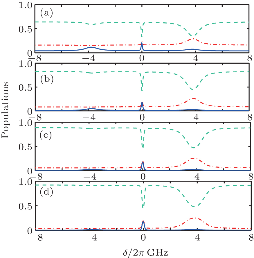 | Fig. 3. The steady-state populations of the qubits states vary as the two-photon resonance detuning δ for κ = 0.08g, γ = 0.05g, J = 3.8 (2π GHz) and pumping rate (a) p = 0.2g, (b) p = 0.5g, (c) p = 0.8g, (d) p = 1.2g. The curves correspond to the populations of state | ↑ ↑ 〉 (green dashed lines), | + 〉 (red dot– dashed lines), and | ↓ ↓ 〉 (blue solid lines) respectively. |
All above we discussed the coupled qubits’ properties and found that two-photon emission can be realized by choosing appropriate parameters. Now we analyze the resonator’ s properties. We bring in three typical variables to describe the resonator field: (i) the mean number of the photons 〈 n〉 , (ii) the Fano factor, which describes the fluctuations of the photon number, and it is defined as[45]

where n = a† a is the photon-number operator, and (iii) the second-order correlation function at zero delay, which relates to the intensity, can distinguish the nature of the light and quantify the probability of two-photon coincidence detection, and it is defined as[46]

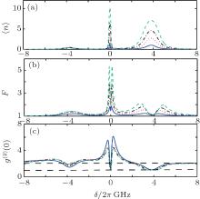
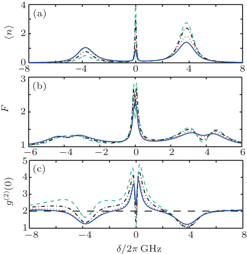
In Fig. 4, by fixing the decay of the qubits and the resonator we display the average photon number, the Fano factor, and the second-order correlation function at zero delay as a function of δ for different values of the pumping rate. There are three peaks of the average photon number, the middle one at two-photon resonance and the other two at one-photon resonances. Generally speaking, the maximum at the two-photon resonance is higher than the one-photon resonances and the right one-photon resonance which corresponds to the transition | ↑ ↑ 〉 ↔ | + 〉 is higher than the left one which corresponds to the transition | + 〉 ↔ | ↓ ↓ 〉 . This behavior is reinforced as the pumping rate is increased. Moreover, the peak at two-photon resonance is narrower than the peak at one-photon resonance as a rule, and it broadens a little with increasing pumping rate. On the other hand, the photon number fluctuations decrease at one-photon and two-photon resonances as the pumping rate increases. At the higher one-photon resonance, F and g(2)(0) are close to unity for large pumping rate while they are still away from unity at two-photon resonance, so there exist large fluctuations in the photon number at two-photon resonance. In the end, both F and g(2)(0) are more than one for all the parameters we consider, and when no resonance happens, g(2)(0) approximates equally to 2 which exhibits a thermal field.
 | Fig. 4. Photon statistics properties of the resonator: (a) Average photon number 〈 n〉 , (b) Fano factor F, and (c) g(2)(0) as a function of the two-photon detuning δ . The parameters are κ = 0.08g, γ = 0.05g, J = 3.8 (2π GHz) and p = 0.2g (blue solid lines), p = 0.5g (red dotted lines), p = 0.8g (dark dot– dashed lines), p = 1.2g (green dashed lines). The horizontal dashed lines in panel (c) indicate the values g(2)(0) = 1 (Poisson distribution) and g(2)(0) = 2 (thermal distribution). |
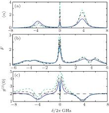
As is shown in Fig. 5, we research the influence of the qubits’ decay rate on the properties of the resonator field. We see that when the decay rate γ is increased, the photon number at main one-photon resonance (the right peak) and two-photon resonance decreases (while the photon number of the left one-photon resonance corresponding to the transition | + 〉 ↔ | ↓ ↓ 〉 increases), and meanwhile the photon-number fluctuations increase (while the photon number fluctuations of the left one-photon resonance decrease). Both F and g(2)(0) are more than one for the parameters we consider.
 | Fig. 5. Photon statistics properties of the resonator: (a) Average photon number 〈 n〉 , (b) Fano factor F, and (c) g(2)(0) as a function of the two-photon detuning δ . The parameters are the same as in Fig. 4 except for a fixed pumping rate p = 0.5g and for different values of the qubit dissipative rate: γ = 0.05g (green dashed lines), γ = 0.1g (dark dot– dashed lines), γ = 0.2g (red dotted lines), γ = 0.3g (blue solid lines). The horizontal dashed line in panel (c) indicates the value g(2)(0) = 2 (thermal distribution). |
To know the influence of the leaks out of the resonator, we study the steady-state properties as a function of the pumping rate for different resonator decay rate at two-photon resonance (δ = 0) in Fig. 6. We conclude that the number of photons inside the resonator increases with the pumping rate increasing and the resonator loss rate reducing. Moreover, it is shown that the Fano factor and the second-order correlation tend to be less than one at κ = 0.02g and κ = 0.05g with the pumping rate increasing while they are always more than one (super-Poissonian field) for all parameters here considered at κ = 0.08g (typical parameter in experiment[30]), and the values of the Fano factor F > 1 are expected in two-photon laser.[47, 48]
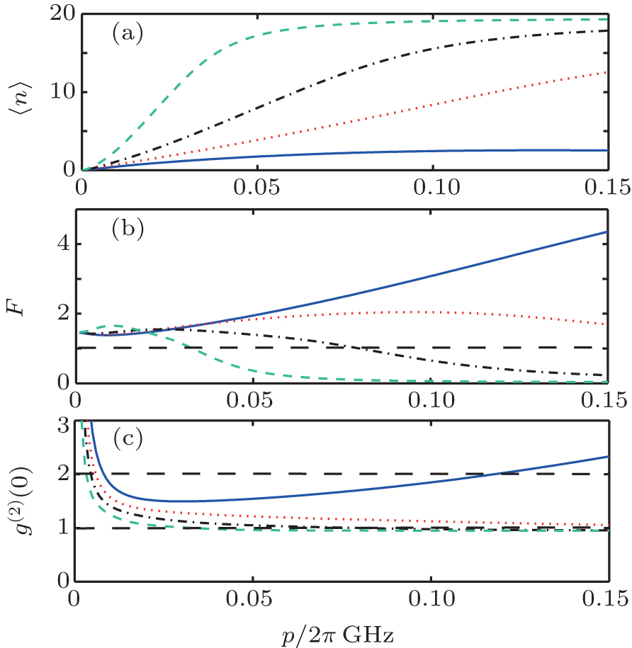 | Fig. 6. (a) Average photon number, (b) Fano factor F, and (c) g(2)(0) as a function of the pumping rate p for δ = 0, γ = 0.05g, J = 3.8 (2π GHz), and different values of the resonator decay rate: κ = 0.12g (blue solid lines), κ = 0.08g (red dotted lines), κ = 0.05g (dark dot– dashed lines), and κ = 0.02g (green dashed lines). The horizontal dashed lines in panels (b) and (c) indicate the value F = 1, g(2)(0) = 1 (Poisson distribution), and g(2)(0) = 2 (thermal distribution). |
At present, we study the steady-state spectral properties of the resonator output. Given a correlation function 〈 a† (τ )a(0)〉 at steady state, we can define the power spectrum as

where 〈 · 〉 equiv Tr (· ρ ss), ρ ss is the steady-state density matrix of the superconducting qubits and resonator. We obtain the spectrum by using the quantum regression theorem[49, 50] and the Quantum Toolbox in Python[51] for various pumping rates at two-photon resonance δ = 0 as shown in Fig. 7.
 | Fig. 7. (a) The common logarithm of spectrum of the resonator output field intensity, (b) the spectrum of the resonator output field intensity in the vicinity of ω − ω a = 0. The parameters are κ = 0.08g, γ = 0.05g, δ = 0, J = 3.8 (2π GHz) and p = 0.2g (blue solid lines), p = 0.5g (dark dot– dashed lines), p = 0.8g (red dashed lines). |
We give the common logarithm of the spectrum for various pumping rates in Fig. 7(a). It displays three main peaks, that is, the middle one at the resonator frequency ω = ω a, the left one at the | ↑ ↑ 〉 ↔ | + 〉 transition frequency, and the right one at the | + 〉 ↔ | ↓ ↓ 〉 transition frequency. It shows that the peak at ω = ω a is dominant and it is almost five orders of magnitude larger than the other two peaks. As the pumping rate increases, the centers of the peaks at one-photon resonances move far away. Figure 7(b) shows the spectrum near ω − ω a = 0. We find that as the pumping rate increases, the number of the resonator photons at ω = ω a increases, the linewidth of the peak decreases and the center of the peak moves close to ω = ω a.
Up to now, what we have discussed shows that the two-photon lasing can be realized at proper parameters. Moreover, two-photon lasers are nonclassical light sources which can be deduced from the effective Hamiltonian (9). Generally, squeezing of a quadrature at the ‘ cavity’ output is usually used to demonstrate the nonclassical characters of the degenerate two-photon lasers. For example, [52] squeezed light is observed for a time when the system is initially in the ground state, the cavity is in a coherent state and the incoherent pumping is added. In this subsection, we also verify such behavior in the system we consider, that is two coupled superconducting flux qubits continuously pumped by incoherent field and strongly coupled to the resonator mode.
Define X = ae− iϕ + a† eiϕ , then the variance of two orthogonal quadrature of the field is Δ X(ϕ ) = 〈 X2〉 − 〈 X〉 2. In Fig. 8, we exhibit the time evolution of the variance of the field quadrature which possesses minimum values at all times by numerical integration of the master equation (4). Initially, the qubits are in the ground state and the resonator is in a coherent state with average photon number 〈 n〉 = 4. The solid lines correspond to the minimum value of the quadrature Δ X(ϕ ) while the dashed lines correspond to the maximum value of the quadrature Δ X(ϕ + π /2), and different colors represent different parameters. We can see Δ X(ϕ )| min < 1 for a period of time indicating that the resonator field becomes squeezed, and the interval of time in which the squeezing appears is longer for smaller rates of the incoherent processes. The squeezing disappears because of the phase diffusion induced by the incoherent processes.
 | Fig. 8. The time evolution of the variance Δ X(ϕ ). The solid (dashed) lines correspond to the minimum (maximum) value of the quadrature Δ X(ϕ ) (Δ X(ϕ + π /2)). The blue lines correspond to κ = 0.08g, γ = 0.05g, p = 0.5g, and the green lines correspond to κ = 0.02g, γ = 0.01g, p = 0.1g. The other parameters are J = 3.8 (2π GHz), δ = 0. The horizontal dashed line indicates the shot-noise limit. |
In summary, we studied the system of two superconducting flux qubits coupled to a superconducting transmission line resonator. It is shown that the coupling between the two flux qubits is necessary for enhancing the two-photon processes and weakening the one-photon processes. We have also studied the steady-state properties of the system: the average photon number, the Fano factor F, and the second-order correlation function at zero delay g(2)(0) for different parameters. Under the condition of two-photon resonance, it is shown that at the parameters which can be achieved in experiment[30] (κ = 0.08g), the Fano factor is larger than one (F > 1), which is expected in two-photon laser, and the spectrum of the resonator output we have displayed shows that the emission of two identical photons is dominant. Besides, the second-order correlation function at zero delay is larger than one (g(2)(0) > 1), which indicates that the resonator field is super-Poisson distribution, and the appearance of the squeezing verifies the nonclassical characteristic of the output field. All that demonstrates that under certain conditions the two-photon lasing can be realized with current technology in circuit QED.
| 1 |
|
| 2 |
|
| 3 |
|
| 4 |
|
| 5 |
|
| 6 |
|
| 7 |
|
| 8 |
|
| 9 |
|
| 10 |
|
| 11 |
|
| 12 |
|
| 13 |
|
| 14 |
|
| 15 |
|
| 16 |
|
| 17 |
|
| 18 |
|
| 19 |
|
| 20 |
|
| 21 |
|
| 22 |
|
| 23 |
|
| 24 |
|
| 25 |
|
| 26 |
|
| 27 |
|
| 28 |
|
| 29 |
|
| 30 |
|
| 31 |
|
| 32 |
|
| 33 |
|
| 34 |
|
| 35 |
|
| 36 |
|
| 37 |
|
| 38 |
|
| 39 |
|
| 40 |
|
| 41 |
|
| 42 |
|
| 43 |
|
| 44 |
|
| 45 |
|
| 46 |
|
| 47 |
|
| 48 |
|
| 49 |
|
| 50 |
|
| 51 |
|
| 52 |
|