
Improved autonomous star identification algorithm*
[Luo Li-Yan† , Xu Lu-Ping, Zhang Hua, Sun Jing-Rong]
, Xu Lu-Ping, Zhang Hua, Sun Jing-Rong]
|
|


†Corresponding author. E-mail: xiaoyan12027@163.com
*Project supported by the National Natural Science Foundation of China (Grant Nos. 61172138 and 61401340), the Open Research Fund of the Academy of Satellite Application, China (Grant No. 2014_CXJJ-DH_12), the Fundamental Research Funds for the Central Universities, China (Grant Nos. JB141303 and 201413B), the Natural Science Basic Research Plan in Shaanxi Province, China (Grant No. 2013JQ8040), the Research Fund for the Doctoral Program of Higher Education of China (Grant No. 20130203120004), and the Xi’an Science and Technology Plan, China (Grant. No CXY1350(4)).
The log–polar transform (LPT) is introduced into the star identification because of its rotation invariance. An improved autonomous star identification algorithm is proposed in this paper to avoid the circular shift of the feature vector and to reduce the time consumed in the star identification algorithm using LPT. In the proposed algorithm, the star pattern of the same navigation star remains unchanged when the stellar image is rotated, which makes it able to reduce the star identification time. The logarithmic values of the plane distances between the navigation and its neighbor stars are adopted to structure the feature vector of the navigation star, which enhances the robustness of star identification. In addition, some efforts are made to make it able to find the identification result with fewer comparisons, instead of searching the whole feature database. The simulation results demonstrate that the proposed algorithm can effectively accelerate the star identification. Moreover, the recognition rate and robustness by the proposed algorithm are better than those by the LPT algorithm and the modified grid algorithm.
Star identification plays an important role in celestial navigation such as the automated sky survey system and the deep space exploration.[1, 2] In the “ lost in space” mode, autonomous star identification is possible to determine the spacecraft attitude[3] without any prior information. In star sensor, the processes of star centroid extraction, star identification, and attitude determination must be performed in real-time, and the accuracy of star identification directly affects the attitude determination of spacecraft. Therefore, the rapid and robust star identification algorithm is required.
During the past few decades, some efforts have been made to study the star identification and many star identification algorithms for star tracking have been achieved. These algorithms have the same goal that is to identify stars as quickly and robustly as possible. The star identification algorithms can be roughly classified into two basic categories:[4] subgraph isomorphism[5] and pattern recognition, [6, 7] in which no prior information about the attitude of the spacecraft is available. In the first type, the stars are treated as the vertices of a graph and the star pair distances or triples (perhaps also including the brightness information) are adopted as the recognition features. For this type of algorithm, it mainly includes triangle algorithm, [8– 11] polygon algorithm, [12– 14] and match group algorithm.[15, 16] As to the other types, some stars or all stars in the field of view (FOV) are used to structure a well-defined pattern. Grid algorithm, [17– 23] neural network algorithm, [24– 27] and genetic algorithm[28– 30] are the representative approaches. Some of the star identification algorithms mentioned above have a lower identification rate, and others are time-consuming. Although many efforts have been made to cope with these problems, there are still a few disadvantages.
The pattern recognition has become a promising trend of star identification in recent years.[31– 34] The log– polar transform (LPT) is rotation-invariant, and it is widely used in moving target recognition, character recognition, etc.[35, 36] Wei et al.[37] have introduced LPT into star identification. They have found that the LPT algorithm is insensitive to positional noise and magnitude noise, and it also has high recognition accuracy when there have been false stars and lost stars. But the circular shift operation must be performed for many times when two feature vectors are compared in the LPT algorithm, which is time-consuming.
In order to reduce the time consumed and enhance the robustness of star identification, we propose an improved autonomous star identification algorithm based on the LPT algorithm. Firstly, the reference star and the alignment star are chosen to reset the new coordinate axes, which make it able to establish the one-to-one relationship between each navigation star and its star pattern. Secondly, all stars observed in FOV are projected onto the new coordinate axes. Then the observed star’ s position in Cartesian coordinates will be converted into polar coordinates by using the LPT. Finally, the feature vector of the star pattern can be achieved according to the LPT result. Compared with the LPT algorithm, the proposed algorithm has no need of the circular shift of the feature vector to find the matching star pattern in the feature database, so it can obtain the identification result quickly. Meanwhile, the logarithmic values of the plane distances between the reference star and its neighbor stars are adopted to form the data of the feature vector, instead of the row numbers in the LPT algorithm, which is more adaptive in practical application. The proposed algorithm has also been compared with the modified grid algorithm to investigate the performance of the proposed algorithm.
The rest of this paper is organized as follows. In Section 2 the imaging principle in the star sensor and the LPT in this proposed algorithm are introduced. In Section 3, the star pattern generation of the proposed algorithm is described in detail. The simulation and analysis are given in Section 4. Finally, in Section 5, the concluding remarks are made.
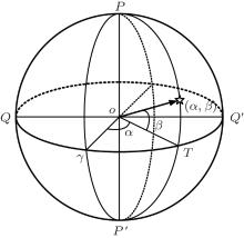
The star catalog and astronomical almanac express a star’ s position in terms of its right ascension α and declination β in the inertial frame (see Fig. 1). The equatorial plane Qγ Q′ and the celestial axis PP′ establish the inertial coordinates. Astronomically, all stars in the sky are located on the sphere whose radius is infinite.
 | Fig. 1. Celestial sphere reference frame. |
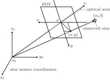
The star sensor is installed on the spacecraft and its coordinates o0x0y0z0 are predesigned. The parallel light from stars impinges on the focal plane of a charge-coupled diode (CCD) (see Fig. 2). In the real image from the star sensor, the star position is expressed in terms of pixels along the x and y axes. A star position in the inertial frame can be converted into a position expressed by the star image coordinates:

where (Nx, Ny is the resolution of CCD in the star sensor, (FOVx, FOVy) is the FOV of CCD, α i, and β i are the right ascension and declination of the i-th star observed respectively, and (α 0, β 0) is the optical axis direction of CCD.
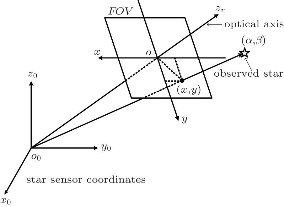 | Fig. 2. Imaging principle in star sensor. |
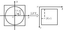
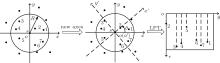
Generally, the LPT is used to extract the rotation invariant feature for image recognition. In the LPT the translation, rotation, and scaling of the image are converted into the displacement variation, which can greatly simplify the problem. Let the star position in Cartesian coordinates be (x, y), then its position (r, θ ) in polar coordinates will be achieved using the following equation:
The process of the LPT is shown in Fig. 3.
 | Fig. 3. The LPT. |
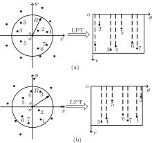
During the process of star identification, one of stars observed in FOV is chosen as the reference star, and it is located at the origin of polar coordinates after the LPT. The observed stars in the neighboring region with a radius R (see Fig. 4(a)) are called the neighbor stars of the reference star. The reference star and its neighbor stars form the pattern of the reference star. In the LPT, the rotation of the stellar image causes the circular shifts of the θ values of stars along the θ axis, and the scaling of the stellar image causes the translations of the r values of the stars along the r axis. Therefore, the LPT results of the patterns of the same reference star are different from each other when the stellar image is rotated. Figure 4 shows the LPT results when the stellar image is rotated and not.
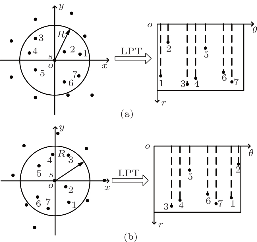 | Fig. 4. The LPT results of (a) the star pattern and (b) when the stellar image is rotated, with the same reference star. |
In the proposed algorithm, some attempts are made to reduce the time consumed in star identification. In order to achieve the unique pattern of the reference star, the centroid coordinates of stars observed in FOV are reset. The nearest neighbor star located within the neighborhood radius R is chosen as the alignment star of the reference star. The direction from the reference star to the alignment star is denoted as the o′ x′ axis among the new coordinate axes (see Fig. 5).
 | Fig. 5. The LPT in the proposed algorithm. |
Let the centroid coordinates of the star observed be (x, y) and (x′ , y′ ) in oxy coordinates and o′ x′ y′ coordinates, respectively, then centroid coordinates of the stars observed in o′ x′ y′ coordinates will be achieved using Eq. (3)

where

is the transformation matrix, θ is the rotation angle from the ox axis to the o′ x′ axis counterclockwise

where (xs, ys) is the centroid coordinate of the reference star (the origin of the o′ x′ y′ coordinates), and (xa, ya) is the centroid coordinate of the alignment star.
And

are the offsets between the origin of the oxy coordinates and the origin of the o′ x′ y′ coordinates, and (x0, y0) is the origin of the oxy coordinates. Generally, x0 = 0 and y0 = 0.
Then the new centroid coordinates of the stars observed in FOV are converted into polar coordinates, and the process in the proposed algorithm is as follows:

The star pattern of the reference star consists of the reference star and its neighbor stars. The rotation invariant feature of the star pattern is extracted by using LPT. The nearest neighbor star of the reference star is chosen as the alignment star. So the centroid coordinate (xa, ya) of the alignment star should satisfy the following condition:

where N is the number of the neighbor stars.
It can be found that the angle between the neighbor star and the alignment star ranges from 0° to 360° . Let the resolution of the θ axis be m in polar coordinates, then the angle interval on θ axis will be 360° /m. The logarithmic value of the plane distance between the reference star and each of its neighbor stars is projected on the r axis in polar coordinates. Let the reference star be s, and assume that the number of neighbor stars whose angles fall in the i-th angle interval is n, then the maximum r value in the i-th angle interval will be expressed as

where θ is the angle between the neighbor star and the alignment star, and the notation ⌈ ⌉ denotes rounding up the value. The angle falling in the i-th angle interval ranges from (i − 1) × 360° /m to i × 360° /m. If there is no neighbor star falling in the i-th angle interval, then ai = 0. The feature vector of the reference stars can be expressed as

The feature vector of each navigation star can be achieved using the method described above, and all these feature vectors form the feature database of the navigation stars.
Let the feature vector of the navigation star in feature database be Ilpt(c), and the feature vector of the star observed in FOV be Ilpt (s), then the similarity between Ilpt (s) and Ilpt (c) is measured by the summation of the absolute difference between the two feature vectors.
where Num is the number of navigation stars. The smaller the summation, the more similar the two feature vectors become.
In order to avoid searching the whole feature database to find the matching star pattern, the number of the non-zero values in the feature vector is used to restrict the search scope. Assume that the number of the non-zero values in Ilpt (s) is Ls, then the feature vectors in the feature database with the number of the non-zero values between Ls– ε 1 and Ls– ε 2 will be compared with Ilpt (s). Therefore, it can quickly obtain the matching result with fewer comparisons instead of the searching for the whole feature database. So the process of identification can be expressed as

where Lc is the number of the non-zero values in Ilpt (c), ε 1 and ε 2 are the tolerances of the number of the non-zero values.
From the above description, the record of each star pattern in the feature database can be expressed as

where id is the index of the navigation star.
The Tycho-2 catalogue is used as the source of our navigation star data. Some stars in the star catalogue, which may lack the lightness information or the location information, cannot be chosen as the navigation stars. Due to the limitation of the resolution of the CCD in the star sensor, it cannot clearly distinguish the two stars when they appear too close. In this paper, two stars less than 20 pixels (about 0.39° ) apart are considered as the binary stars. Therefore, there are 6685 stars to be chosen as the navigation stars whose visual magnitude ranges from 1.0 m to 6.5 m. Each of the navigation stars is regarded as the reference star to construct the feature vector for the onboard feature database. The resolution of the simulated stellar image is 1024 × 1024 pixels with a 20° × 20° FOV. The average number of the stars in FOV is 30.32, with 68 used as the maximum and 3 as the minimum. The experiments are carried out using a microcomputer with a 3.20-GHz Pentium (R) Dual-Core, 1.96-GB RAMS.
The achievable performance of the proposed algorithm is demonstrated via a comparative study between the LPT algorithm[37] and the modified grid algorithm.[20] The simulations mainly include the influences of positional noise, false stars and lost stars on identification, the memory usage, and identification time. The magnitude information about the navigation star is not used in the proposed algorithm, so the influence of the magnitude noise on star identification is ignored.
As is well known, a lot of geometric information about the observed stars located on the edge of FOV is lost. In order to obtain the geometry information out of the observed stars as much as possible, the observed stars near the center of FOV are chosen as the reference stars in this paper. The identification process is considered to be unsuccessful when the number of stars observed in FOV is less than 3.
It can be known from Ref. [37] that the recognition rate changes with the variation of the neighborhood radius R and it can achieve the highest recognition rate when R = 6° . So the neighborhood radius R is set to be 6° throughout this paper. The resolution of the θ axis in polar coordinates denoted by m is set to be 100. In the process of star identification, the tolerances of the number of the non-zero values are set to be ε 1 = ε 2 = 1 in experience.
The positional noises are added to the real centroid coordinates of star points in the simulated stellar image to investigate the robustness of the identification algorithm.
Figure 6 shows the recognition rates of the three star identification algorithms in which only the positional noises are added. The results show that the proposed algorithm has a better anti-noise ability than the LPT algorithm and the modified grid algorithm. The recognition rate of the proposed algorithm is up to 98.04% when the positional noise is 0.5 pixels, while the recognition rate of the LPT algorithm is just about 91.76% and the recognition rate of the modified grid algorithm is about 97.61% under the same condition.
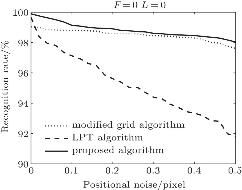 | Fig. 6. Recognition rates versus positional noise (F: false star, L: lost star). |
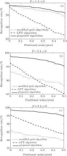
Space debris and spacecraft may be mistaken as the observed stars (false stars), which will disturb the star identification. In this section, false stars will be added on the simulated stellar image to verify the performance of the proposed algorithm. Figure 7 shows the statistical results of the recognition rates of the three algorithms for all 6685 navigation stars with the number of false stars ranging from 1 to 3. The false stars are randomly distributed on the simulated stellar image.
In Fig. 7, without positional noise, the identification rate of the proposed algorithm decreases from 99.08% to 98.55% when the number of false stars increases from 1 to 3. Under the same conditions, the rate of the LPT algorithm decreases from 98.47% to 95.46%, and the rate of the modified grid algorithm decreases from 99% to 86.5%. It can be found that the recognition rates of the three algorithms decrease by 0.53%, 3.01%, and 12.5%, respectively. It can be known from the analysis results that the LPT algorithm is more sensitive to positional noise than the other two algorithms, and the false stars greatly affect the recognition rate of the modified grid algorithm. The proposed algorithm outperforms the LPT algorithm and the modified grid algorithm when there are false stars.
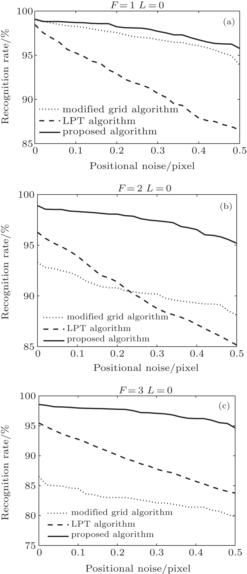 | Fig. 7. Recognition rates versus positional noise for the cases of 1 (a), 2 (b), and 3 (c) false stars. |
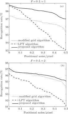
Some stars in the sky may not be captured by CCD (lost stars) because of the shelter of other spacecraft or the hardware failure of the star sensor. In tests, the stars observed on the simulated stellar images are deleted randomly. Figure 8 shows the influences of lost stars on star identification. From the results it can be found that the LPT algorithm is sensitive to lost stars, while the proposed algorithm performs well. The downtrend of the recognition rate of the modified grid algorithm is similar to that of the recognition rate of the proposed algorithm, but the robustness of the proposed algorithm is better than that of the modified grid algorithm.
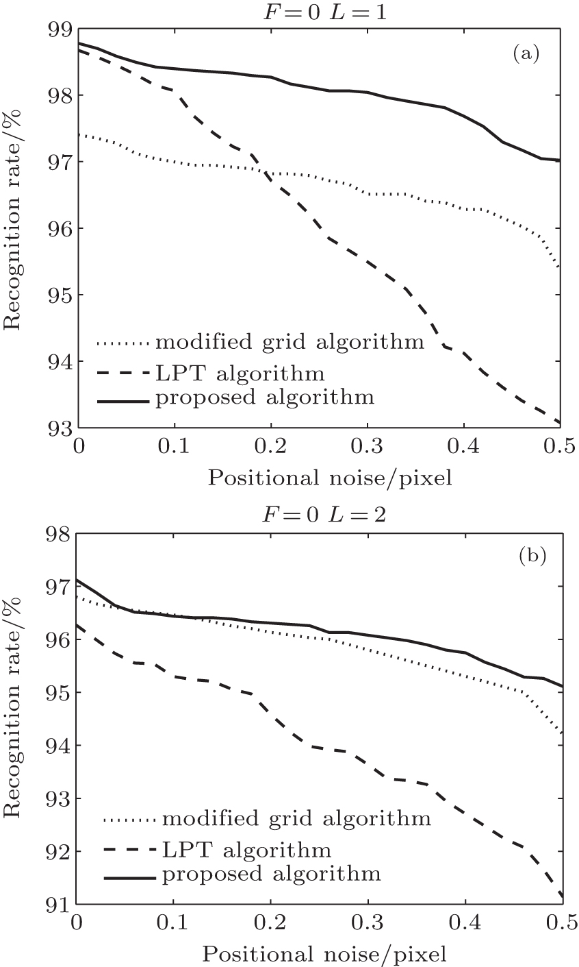 | Fig. 8. Recognition rates versus positional noise for the cases of 1 (a) and 2 (b) lost stars. |
To sum up, even under positional noise, as well as the existence of false stars and lost stars, the proposed algorithm is more robust than the LPT algorithm and the modified grid algorithm.
The identification time and memory usage are the important factors in actual implementation of the star identification algorithm. The simulation results are summarized in Table 1.
| Table 1. Benchmarking of star identification algorithms. |
In the LPT algorithm, the comparisons between the feature vector of the reference star and the feature vector in the feature database are considered as the string matching. The rotation of the stellar image will cause the translation of the logarithmic values of star plane distances along the θ axis, so the feature vector of the reference star needs the circular shift for many times when it is compared with each feature vector in the feature database. It is known that the string matching involving circular shift costs a lot of time. Meanwhile, it needs to search the whole feature database to find the identification result. So the LPT algorithm is time-consuming.
The modified grid algorithm requires the logical AND operations when two star patterns are compared, and the recognition time increases obviously with the increase of the number of the grid cells. It also needs to search the whole feature database to find the best matching pattern.
The proposed algorithm resets the coordinates by using the reference star and the alignment star, and the star pattern is invariable when the stellar image is rotated. Thus there is no need to find the matching feature vector in the feature database for the circular shift of the feature vector, which accelerates star identification. Meanwhile, the number of the non-zero values of the feature vector is used to narrow down the search scope, which makes it able to obtain the identification result with fewer comparisons.
The proposed algorithm has an average identification time of 7 ms, while the LPT has an average identification time of 73.8 ms, which is about 10 times that of the proposed algorithm. The average identification time of the modified grid is longest (0.4017 s). Each logarithmic value in the feature vector of the proposed algorithm occupies 2 bytes, and each value in the feature vector of the LPT algorithm just occupies 1 byte. So the feature database of the proposed algorithm with 1.3 MB is larger than that of the LPT algorithm with 0.65 MB. Because the modified grid algorithm needs to store the star pattern, its feature database is largest (7.38 MB). Although the feature database of the proposed algorithm is larger than that of the LPT algorithm, it is acceptable in practical application.
The experimental results validate the theoretical analysis. Despite the fact that the memory requirement for our algorithm is more than that of the LPT algorithm, it is supported by the available hardware. As such, its practical application is feasible.
Compared with the LPT algorithm, the proposed algorithm avoids the circular shift operation which greatly reduces the star recognition time. At the same time, it also effectively enhances the robustness of star identification. The centroid coordinates of observed stars are reset, with the result that the navigation star has the same feature vector, whether the stellar image is rotated or not. Therefore, the comparison between the two feature vectors can be simplified into the subtraction operation. The simulation results confirm that the proposed algorithm is much more time-saving than the LPT algorithm and the modified grid algorithm. Even under positional noise, as well as with the existence of false stars and lost stars, the proposed algorithm performs better than the LPT algorithm and the modified grid algorithm in terms of identification time, recognition accuracy, and robustness. Although the feature database of the proposed algorithm is larger than that of the LPT algorithm, it is supported by the available hardware.
| 1 |
|
| 2 |
|
| 3 |
|
| 4 |
|
| 5 |
|
| 6 |
|
| 7 |
|
| 8 |
|
| 9 |
|
| 10 |
|
| 11 |
|
| 12 |
|
| 13 |
|
| 14 |
|
| 15 |
|
| 16 |
|
| 17 |
|
| 18 |
|
| 19 |
|
| 20 |
|
| 21 |
|
| 22 |
|
| 23 |
|
| 24 |
|
| 25 |
|
| 26 |
|
| 27 |
|
| 28 |
|
| 29 |
|
| 30 |
|
| 31 |
|
| 32 |
|
| 33 |
|
| 34 |
|
| 35 |
|
| 36 |
|
| 37 |
|