The capability of laser radiation to control the translational degrees of freedom has intensively been studied for several decades. These studies offer a wide spectrum of important applications and useful theoretical models.^{[1, 2]} The mechanical action of light is used for the deep laser cooling of both neutral atoms and charged atomic ions as well as for the trapping of neutral atoms. Electromagnetic traps (similar to the Paul or Penning traps) are conventionally used for the ion confinement.

Recently the interest has arisen from the problem of all-optical trapping of ions, i.e., from ion trapping without applying radiofrequency or electrostatic and magnetostatic fields.^{[3, 4]} Unfortunately, the shallow depth Δ W_d of monochromatic dipole trap (ODT) or optical lattice (OL) can be a serious obstacle for their use in the trapping of a few ions due to the Coulomb repulsion of ions (although ODT and OL are quite successfully used for all-optical trapping of neutral atoms^{[2, 5– 7]}).

An alternative method for long-time trapping of the interacting ions, the confinement of the ions in a three-dimensional (3D) dissipative polychromatic optical superlattice (OSL), ^{[8, 9]} was considered in Ref.  [4]. The action of such a 3D OSL (with the spatial period ∼ L greatly exceeding the light wavelength λ , L ≫ λ ) on the ions is based on the effect of the gradient (dipole) force rectification in the non-monochromatic (bichromatic, polychromatic) optical fields.^{[10– 12]} Due to unique features of the rectified gradient force RcGF, ^[10] OSL is capable of inducing 3D superdeep (as compared with ODT or OL) potential wells (for the ions) with the value of depth

where ħ Δ _s is the characteristic value of the light (Stark) shifts of ionic levels. Moreover, the light-induced friction force is exerted on the ions in OSL, resulting in the cooling of ions. The computer simulation results of the ion motion in OSL (for the case of two ytterbium ions) presented in Ref.  [4] demonstrate that the OSL action on the ions can lead to their deep cooling and to the formation and long-time confinement of the two-ion (Coulomb) cluster. Such a cluster has an approximately fixed (with the accuracy up to small fluctuations) interionic distance (size) and the center-of-mass (CM) position. Note that in the considered two-ion system all the main factors hindering the all-optical ion trapping are present: the Coulomb repulsion, quantum fluctuations of the optical forces, ^{[1, 13]} and finite depth of the light-induced potential wells.

The analysis of the computer simulation results allows one to formulate the following conditions for the long-lived two-ion cluster formation within a single unit cell Ω ₀ of OSL.^[4]

There must exist equilibrium points {η * } in the six-dimensional configuration space (of the ion spatial positions {η } = (r₁, r₂)), where the Coulomb repulsion of ions is balanced by the trapping force (RcGF F_0R in our model) and the total potential energy U_t({η }) achieves a local minimum, i.e., a point where

where α = 1, 2, r_α is the position of the α -th ion, U_R is the potential of RcGF, U_c(r) = e²/4π ε ₀r is the Coulomb energy of two ions separated by the distance r, e is the ion charge, d²U_t({η * }) is the second differential of U_t({η }) at the point {η * }.

There exist equilibrium cluster configurations {η * } if the value of the light-induced potential well depth Δ W is sufficiently large as compared with the Coulomb energy U_c(L):^[4]

where L is the spatial period of OSL.

The cluster configuration {η * } is metastable^[4] due to the quantum fluctuation of the optical trapping force. Notably, the metastable-state lifetime τ _M is a strongly increasing function of the ratio of the potential well depth Δ W to the effective cluster temperature T, which is established by the balance between the optical cooling of the ions and their heating due to the optical force fluctuations. Therefore, another important condition for the formation of the long-lived cluster in OSL can be presented by the inequality

where T is expressed in energy units. Inequality  (4) also provides the smallness of the random fluctuations of the interionic distances (at the time points t < τ _M).^[4]

The presented conditions seem perfectly natural and simple for the interpretation. However they are valid only in the approximation of slow ions (SI), i.e., in the case of

where is the thermal velocity of the ions, m is the ionic mass, and v_c is the so-called capture velocity^[2] determining the region (in the velocity space) of the most efficient action of the optical forces, outside this region the forces decrease rapidly with increasing ion velocity. The SI approximation and the quasi-classical theory of optical forces^{[1, 13]} allow treating the ion motion in OSL as the Brownian motion under the action of conservative trapping force (RcGF).^[4] In this model, neither the friction coefficient nor the diffusion coefficient depends on ion velocity v.

The present paper considers a new model where the parameter ε is not small enough and an explicit velocity dependence of RcGF, friction and diffusion coefficients are taken into account.

The necessity for the special analysis of this model is due to the following important circumstances. The low (sub-Doppler) limit of the ionic temperature in OSL is achieved at the low intensity of the optical field and is accompanied by the violation of condition  (5).^[9] The velocity profile of RcGF is determined (see e.g. Refs.  [10], [12], and [14]) by the multipliers of the ℒ (v_j/v_c) type, where v_j are the velocity projections onto the axis j ∈ {x, y, z}, and ℒ (u) is the Lorentzian function:

Therefore, RcGF is a non-conservative force, and equation  (1) and condition  (2) (as well as the outcoming relation  (3)) loose their senses at ε ∼ 1 and do not allow one to unambiguously predict possible equilibrium configurations of the two-ion cluster. The metastability condition  (4) is also difficult to explain since it is not understandable in advance how to determine accurately the height of the energy barrier preventing the cluster from decaying in the case of the non-conservative RcGF.

Finally, a reasonable question arises. Is it at all possible in this case (i.e., at ε ∼ 1) to form in OSL a long-lived Coulomb ion cluster which is similar to that predicted by the computer simulation in Ref.  [4].

Our answer to this question of principle is “ yes” , and a correct formulation of the basic conditions for the formation of such a cluster in OSL is given. These conditions (with an arbitrary value of ε ) can be written in the form analogous to relations  (1)– (4), where it is, however, necessary to perform suitable renormalization (re-definition) of the parameters and forces. In particular, for renormalization of the Coulomb interaction it is necessary to replace the charge e (in the expression for U_c(r)) by the effective (renormalized) charge e* :

where e* is the function of the governing parameters of OSL, χ , and G.^[9]

In other words, one shows that with the arbitrary value of the parameter ε and the time scales larger than the inverse friction coefficient ϰ ^{− 1}, the light-induced Brownian motion of the ions in the configuration space {η } can be described using a renormalized SI model.

Our analysis is based on the asymptotic expansion of the Wigner distribution function (for the ions in OSL) in the Knudsen number of problem^[9]

where λ _r ∼ sϰ ^{− 1} has the meaning of the effective free-path length of the ions in a viscous “ fluid” of photons.

Another interesting aspect (not only for optical physics but also for statistical mechanics (e.g., see Ref.  [15]) of the problem under consideration is connected with the non-Maxwellian characteristic of the velocity distribution of ions in OSL. It is shown that the main part of the velocity distribution can be well approximated by the 3D Tsallis distribution

where exp_q(v²) = [1 + (q − 1)v²]^{1/1− q} is the so-called q-Gaussian, normalizing factor N, and the index q and T₀ each are a function of the governing parameters of OSL.

In this section the equations of the ion motion in the configuration space {η } = (r₁, r₂) are derived. These equations are to be used further to obtain correct conditions for the formation of the metastable two-ion (Coulomb) cluster in OSL when inequality  (5) is violated. The overdamped characteristic of the ion motion in OSL, which is expressed by inequality  (8), Kn ∝ ζ ≪ 1, allows using the method of Chapman– Enskog type (e.g., see Refs.  [20] and [21]) for finding the solution of Eq.  (18) on a diffusion time scale .

Taking into account the results of the previous section it is possible to reformulate the formation conditions of the two-ion (Coulomb) cluster in OSL (see Eqs.  (1)– (4)) by substituting the “ bare” Coulomb force and RcGF by the renormalized forces. The influence of this renormalization appears to be rather significant for the OSL parameters which correspond to the minimum ion temperatures (see Subsection  3.2): 𝒜 ∼ 3, g ≫ 1. Indeed, the effect of renormalization can be ignored if the corrective multipliers Λ _c and Λ _sp are close to unity: Λ _c ≈ 1 and Λ _sp ≈ 1, i.e., when

Note that this condition is equivalent to inequality  (5).

Inequality  (48) imposes rather strong constraints on the governing parameters G and χ and is unlikely to be satisfied at 𝒜 ∼ 3. Figure  2 illustrates the dependence of the renormalized charge e* on the parameter G for the case of the ¹⁷¹Yb⁺ ions (γ = 4.81 × 10⁷ s^{− 1}, λ = 370  nm). One can see from Fig.  2 that the effective charge e* can exceed the “ bare” charge by more than 1.5 times and, consequently, the effective Coulomb force ∝ (e* )² can increase several times in comparison with the “ bare” Coulomb force.

Fig.  2.

Figure Option ViewDownloadNew Window

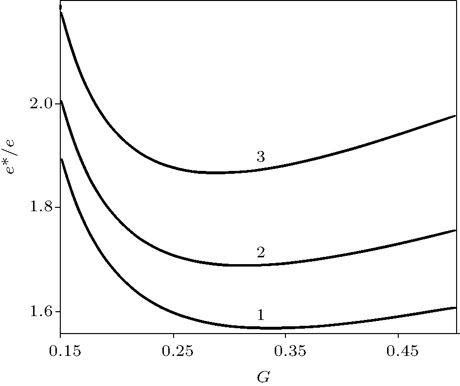Fig.  2. Ratios of the effective (renormalized) ion charge to the “ bare” charge versus G. The governing parameter of OSL G = Gi (for i ∈ {x, y, z}) is proportional to the intensity of the “ far-off-resonant” field, which is in accordance with Eq.  (16). The governing parameter of OSL χ is proportional to the intensity of the resonant field E′ , χ = 0.07 (line 1), χ = 0.06 (line 2), χ = 0.05 (line 3). The OSL and ion parameters are , b = 5, γ = 4.8 × 107  s− 1, m = 171  a.u. (The units a.u. is atomic unit), and λ = 370 nm. The parameter 𝒜 = 3 at G ≈ 0.17 and 𝒜 = 9 at G = 0.5.

The equations of the force balance (compared with Eq.  (1)) should be rewritten as follows:

where α ∈ {1, 2}, i ∈ {x, y, z}. According to Ref.  [4], we introduce relative and center-of-mass coordinates {η } → {η ₁} = (r, R):

For certainty, the situation is considered when two ions are located in the same OSL unit cell Ω ₀, with the center of the cell Ω ₀ coinciding with the origin of coordinates. Then, the equilibrium (metastable) configurations of the ion cluster are determined by the following relations which result from the minimization of the effective total potential energy Ŭ ^eff(η ₁)) and from the second-order condition for the minimization of Ŭ ^eff(η ₁):

where , H_ii and h_ii are the non-zero elements of the Hessian matrix for the equilibrium i-configuration of the ions oriented along the i axis,

Inequality (53) implies that the second differential of Ŭ ^eff({η ₁}) at the point has a positive-definite quadratic form. For each fixed index i ∈ {x, y, z} equation  (51) and condition  (53) allow us to find the equilibrium i-configuration . Since p_x = 1, and p_y, p_z > 1, then, the deepest light-induced wells are the wells along the x axis. Thus, the stable cluster configurations (at least, x-configurations) can appear only if the potential well depth along the x axis is sufficiently large as compared with the Coulomb energy Ŭ _c(L):

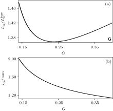
Indeed, in this case there is the positive root ξ * < 1/4 of Eq.  ( 51) for i = x (p_x = 1) and the elements of the Hessian matrix are positive (H_xx, H_lx, h_xx, h_lx > 0, l ∈ {y, z}), i.e., condition  (53) is satisfied. When inequality  (48) is satisfied, condition  (55) is transformed into earlier obtained condition  (3).^[4] It follows from Eq.  (55) that the formation of the two-ion cluster is only possible in the case where the period of OSL exceeds the critical length (L > L_cr) at which . Since ξ * < 1/4, then the critical (minimal) size of the cluster (i.e., interionic distance) l_cr is equal to L_cr/2.

It is easily understood if it is taken into account that Ŭ _c(1) ∝ 1/L and and l_cr = 2L_crξ * . In the present paper a physical situation is investigated when the effects of the nonlinear dependence of the optical forces on the ion velocity are manifested and, thus, inequalities  (5) and (48) are not satisfied. In this case, Λ _c/Λ _R > 1 and the critical period L_cr exceeds its value corresponding to the SI model. It is a result of the renormalization of the bare ion charge and Coulomb interactions due to the nonlinear velocity dependence of the optical forces. Figure  3 demonstrates the appreciable increase of the critical period in the renormalized model in comparison with the model of the slow ions.

Fig.  3.

	Figure Option ViewDownloadNew Window
	Fig.  3. (a) The ratio of the normalized critical OSL period Lcr to the critical OSL period in the “ bare” SI model versus the governing parameter of OSL G. (b) The critical size of the two-ion cluster versus the parameter G. The governing parameter of OSL χ = 0.07, all the other parameters are the same as those in Fig.  2.

The condition analogous to inequality  (4) for the renormalized model is modified to the following inequality:

Inequality (56) provides a possibility of forming a long-lived two-ion cluster with the lifetime τ ∼ τ _M ≫ τ _cl, where τ _cl is the characteristic time of the cluster formation.^[4] Besides, from inequality (56) it follows that at time τ ≫ τ _cl the fluctuations of the ions about their equilibrium positions are small as compared with the dimensionless cluster size 2ξ * .

Now we consider the last question in more detail. To be more exact, we are to investigate the dynamics of the fluctuations of ions about their equilibrium positions corresponding to x-configuration with p_y = p_z > 1. The linear approximation of Eq.  ( 45) can be written in the compact matrix form

where ℋ is the diagonal Hessian matrix (ℋ = Diag(h_xx, h_xy, h_xz, H_xx, H_xy, H_xz)) which is defined by Eq.  (54) with i = x, p_y = p_z = p > p_x = 1, r̃ is the column vector, r̃ = col(r̃ _x, r_y, r_z, R_x, R_y, R_z), r̃ _x = r_x − ξ * , and ξ * is the positive root of Eq.  (51) for i = x,

is the Gaussian white noise (i ∈ {x, y, z}, β ∈ {+ , − }) and correlator .

Equation  (57) can be used for the time shorter than the characteristic lifetime of the ion cluster τ _M, whose finiteness is due to the manifestation of the large rare fluctuations, ^[22] i.e., the cluster metastability. This equation leads to the estimation of the characteristic formation time of the cluster with h = min{H_xx, h_xx, h_yx = h_zx}. The numerical simulations^[4] indicate that under condition  (56) the following is always true: τ _M ≫ τ _cl. Using the standard method of the analysis of stochastic differential equations^{[19, 22]} one can easily obtain (established when τ _cl ≪ τ < τ _M) quasi-steady values of the average and standard deviation σ for the column vector r̃ components.

In particular, the following important relations are obtained:

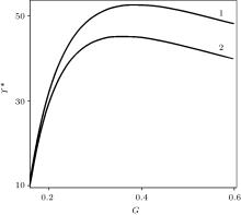
where δ r = σ {| r| }/2ξ * and δ R_i = σ {R_i}/2ξ * are the values characterizing the relative level of fluctuations (which is compared with the size of the cluster 2ξ * ), the interionic distance, and CM position. These fluctuations are suppressed when the parameter ϒ * increases. Figure  4 shows the characteristic scale of the value of ϒ * for certain values of the OSL parameters. For the parameters in Fig.  4 the δ r and δ R_i are about 0.07, temperature T ≈ 0.3, 8.5 > 𝒜 > 2.65 and the coupling parameters, Γ _c, , considerably exceed unity: Γ _c = Ŭ _c(2ξ * )/T ≈ 60, at G ≈ 0.28. Moreover, in this case the parameters of the expansion of the DF, ζ ₁, ζ ₂, are significantly lower than unity: ≲ 0.05, the intensity of the partially coherent optical field I′ does not exceed the value 40  mW/cm², and intensity of the “ far-off-resonant” field I_i ≲ 1  W/cm² for Δ _y ∼ 1.5Δ _x, Δ _z ∼ 2Δ _x, Δ _x ∼ 80γ , Γ = 10γ .

Fig.  4.

	Figure Option ViewDownloadNew Window
	Fig.  4. The parameter ϒ * versus the governing parameter of OSL G. The value of ξ * is fixed to be equal to 0.18, the governing parameter of OSL χ = 0.07 (line 1), χ = 0.0.5 (line 2). All the other parameters are the same those as in Fig.  2.

This example demonstrates a real possibility to satisfy all the formation conditions of the two-ion (Coulomb) cluster in OSL in the case where the SI approximation (inequality (5)) is not applicable and one has to use the renormalized model constructed in the present work.

It is shown that in order to correctly formulate the conditions for the formation of the two-ion (Coulomb) cluster in the 3D polychromatic dissipative superlattice cell, suitable renormalization of the optical and Coulomb force terms in the force balance equation is necessary. Such a renormalization allows one to take into account the important factor of the nonlinear dependence of the optical forces on the velocity and, the strongly non-Maxwellian (Tsallis type) characteristic of the velocity distribution of ions in OSL.

The renormalization effects are most significant for the case of weak light fields, where the lowest (sub-Doppler) temperatures of ions are reached. In this case the effective charge e* (which determines the renormalized Coulomb ion– ion interaction) is a function of OSL governing parameters, G and χ , and always exceeds the value of the “ bare” ion charge. The consequence of this circumstance is the increase of the critical (minimal) period of the OSL at which the effect of the two-ion cluster formation is achieved.

Another important result of the present work which has stand-alone value, is the derivation of a closed system of stochastic differential equations describing the light-induced Brownian motion of ions in the configuration space (r₁, r₂). This system of reduced Langevin equations with additive noises is considerably simpler than the original system of the Langevin equations with multiplicative noises. Using these equations to describe the ion dynamics in OSL is not limited to the narrow frames of the slow ion approximation^[9] and allows implementing the numerical simulations of the long-time dynamics of the ions for much longer time than in Ref.  [4]. This is extremely important for the investigation of the dependence of the cluster life-time on the OSL parameters. The cluster life-time is determined by the rare large fluctuations, thus, its accurate calculation requires carrying out simulations in long-time intervals.

In conclusion, it may be suggested that the considered effect of renormalization of the Coulomb interaction should be used in problems of the optical creation and confinement of ultracold electron– ion plasma.^[8]