


Photodetachment microscopy of H− in the magnetic field near different dielectric surfaces*
[Tang Tian-Tian† , Zhang Min, Zhang Chao-Min]
, Zhang Min, Zhang Chao-Min]
|
|


†Corresponding author. E-mail: tangtiantian198512@163.com
*Project supported by the Natural Science Foundation for Youths of Shandong Province, China (Grant No. ZR2014AQ022).
We study the photo-detachment interference patterns of a hydrogen negative ion in the magnetic field near different dielectric surfaces with a semi-classical open orbit theory. We give a clear physical picture describing the photo-detachment of H− in this case. The electron flux distributions are calculated at various dielectric surfaces with unchanged magnetic field strength. It is found that the electron flux distributions of H− are very different in a magnetic field near different dielectric surfaces, namely the dielectric surface has a great influence on the photo-detachment interference pattern of the negative ion. Therefore, the interference pattern in the detached-electron flux distribution can be controlled by changing the dielectric constant. We hope that our studies may guide the future experimental research in photo-detachment microscopy.
Photo-detachment microscopy is used to measure the electron affinities of atoms and molecules with unprecedented accuracy. In the early 1980s, Demkov, Kondratovich and Ostrovsk introduced the principle of photo-detachment and photo-ionization microscopy.[1, 2] They suggested that during the detachment of an electron from a negative ion in the presence of an electric field, the electron would be able to follow several trajectories to the detector, and that this situation would produce an interference pattern. They studied the microscopy theoretically and discussed the possibility of an experiment on the photo-detachment or photo-ionization process in the presence of an electric field. The first experimental implementation of photo-detachment microscopy was made by Blondel et al.[3] Ejected electrons produced by photo-detachment of Br− in electric fields were recorded on a high resolution detector perpendicular to the applied electric field. The recorded pattern displayed concentric interference fringes. A subsequent observation of photo-detachment of O− in an electric field was also performed by the same group.[4] The experimental results were supported by the quantum calculation of Kramer et al.[5] On the other hand, Du developed a semi-classical method to predict outgoing electron current distributions in photo-detachment of H− in the electric field.[6] An analytical formula for the electron flux distribution has been presented. The oscillations in the spatial distribution of detached-electrons are attributed to the interference of waves propagating along two distinctive paths from the region of the bound state of H− to the same point. The method of Du may be extended to treat more complicated negative ions. Recently many investigations of the electron dynamics and the photo-detachment microscopy in parallel electric and magnetic fields have been reported by Bracher et al.[7, 8] and Bracher and Delos.[9]
Lately, Zhao and Delos[10, 11] developed theories and numerical methods for photo-ionization microscopy of hydrogen atoms in strong electric fields, in semi-classical and quantum-mechanical frameworks respectively. Semi-classical open-orbit theory is presented to describe the macroscopic-distance propagation of outgoing electron waves. Spatial distributions of electron probability densities and current densities are predicted. The open-orbit theory, based on an assumption that electron waves propagate along classical paths from a point-like source to a detector, provides a clear and intuitive physical picture to explain the structures of observed geometrical interference patterns in photo-ionization microscopy.[10] In our previous work, we have studied the electron flux distribution of H− in a magnetic field near a metal surface using an open-orbit theory.[12] We mainly studied the effect of the changed magnetic field on the electron flux distribution, and interference patterns were obtained. In the present paper, we study the photo-detached microscopy of a hydrogen negative ion in the magnetic field near a dielectric surface by the same theory. But we pay particular attention to the interference patterns in the flux distributions on the detector with different dielectric surfaces. It is found that the electron flux distribution of H− can be modified sensitively by the dielectric constant. This subject is interesting, and has potential applications in many important research fields, including surface catalysis and generation of ultrafast lasers. It is an even more accurate method of measuring electron affinity and a controlled interaction of the very low energy photoelectrons with specific regions of the surface. We hope that our studies may guide the future experimental research on the photo-detachment microscope of the negative ions in the presence of external fields and surfaces.
On the basis of semi-classical open orbit theory, [10] the physical picture of the photo-detachment process of H− in the magnetic field near a dielectric surface can be described as follows. When the laser is on, the negative ion may absorb a photon of energy Eph and the detached electron becomes an outgoing p-wave. The wave then propagates away from the hydrogen atom in all directions, following classical trajectories. As the electron moves far from the ions, the wave functions can be constructed using the semi-classical approximation. Whenever two or more trajectories of the detached electron arrive at a given point on the detector, the corresponding waves interfere constructively or destructively, thus creating an interference pattern in the electron flux distribution on the detector. In order to calculate the electron flux distribution at a given point on the detector, we must find all the trajectories of the detached electron which go through that point in great detail.
The schematic plot of the system is given in Fig. 1. As in the previous studies, [12, 13] H− is regarded initially as a one-electron system loosely bound by a short-range, spherically symmetric potential of the hydrogen atom. A z-polarized laser is used for the photo-detachment and the distance between the dielectric surface and the negative ion is d. An external magnetic field B perpendicular to the dielectric surface is applied. A position-sensitive detector is placed in the plane at z = − z0 . According to the electrostatic image method, [14] the potential acting on the active electron in the ion– surface system can be described as V = Vb + Vc + Vi, in which Vb and Vc are both short-range potential, then can be ignored after the electron has been detached. Vi is the interaction potential between the detached electron and the image electron e′ = α E, which is a Coulomb-like attractive image potential: Vi = − α e2/4(d + z), α = (ɛ − 1)/(ɛ + 1) > 0, ɛ is the dielectric constant. (In our paper, α also represents the dielectric constant value.) Therefore, the Hamiltonian for the detached electron in the magnetic field near a dielectric surface has the following form (in cylindrical coordinates and atomic units: a.u.)[14, 15]

In which ω L = B/2c is the Larmor frequency, B is the magnetic field strength, c is the speed of light, and α /4d is an additional term to ensure V(z = 0) = 0, which has no influence on the photo-detachment process.[16] The Hamiltonian can be divided into the motion along the z axis and the motion in the x– y plane due to the cylindrical symmetry of the system. Take the angle included between the initial outgoing direction and the z axis to be θ out, the motion equation of the detached-electron in the ρ direction becomes

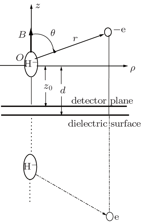 | Fig. 1. Schematic plot of the H− in the magnetic field near a dielectric surface. The magnetic field is along the + z axis. H− is at the origin. |
The motion in the ρ direction is the same as the cyclotron motion in the magnetic field. The cyclotron period is tc = π /ω L . Since the ion– surface potential is an attractive one, the motion of the detached electron along the z axis is like the case of an electron moving in an electric field. We cannot give the motion equation of the detached electron along the z direction by a concise formula, but we can obtain the time tz for a detached-electron to reach the detector perpendicular to the z axis at z < 0: (A detailed derivation of this equation is shown in Appendix A.)
When tz = ntc (n is a positive integer), the detached-electron collides with the detector. For a given point on the detector, there exist several electron trajectories passing through it. Some classical trajectories of the detached-electron hitting the detector at a given point are shown in Fig. 2. We can see that each classical trajectory corresponds to an outgoing electron angle.
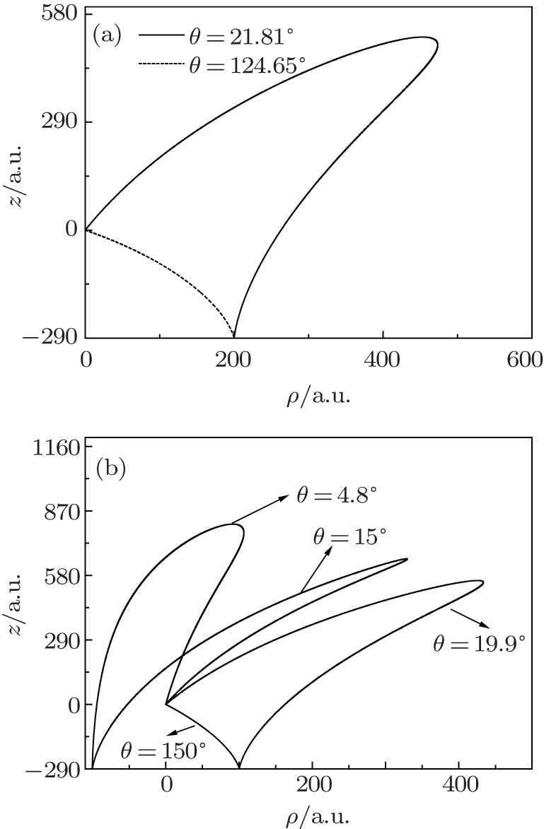 | Fig. 2. Some classical orbits of the detached electron reaching the detector with the magnetic field strength B = 10 T. (a): There are two classical orbits at the point (200 a.u., − 290 a.u.) with the ejection angles θ = 21.81° and 124.65° respectively. (b): There are four classical orbits at (| ρ | = 100 a.u., z = − 290 a.u.) with the ejection angles θ = 19.9° , 150° , 4.8° , and 15° respectively. |
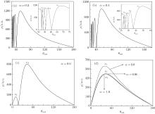
When the electron reaches the detector, we record the final value of the cylindrical coordinate ρ i(θ out) and call it collision radius.[10] As a matter of fact, equation (2) gives the absolute value of ρ i (θ out). By substituting time in Eq. (3) into ρ in Eq. (2), the curve parameterized by angle θ out from 0 to π is the θ out– ρ diagram. A curve of the final position at the detector ρ i versus θ out is shown in Fig. 3, Ci is the boundary point.[17] Next, we use θ out– ρ diagram to find the typical trajectories and to analyze the detached-electron dynamics. The diagrams will be useful in understanding the structures in the detached-electron flux on the detector because the number of intersection points between a θ out– ρ curve and a line defined by ρ = constant gives the number of orbits arriving at the same point ρ on the detector. In the following calculations, we keep the ion– surface distance d = 300 a.u. (the unit a.u. expresses the atomic unit) and electron energy E = 0.01 eV unchanged. The detector is placed in the plane at z = − 290 a.u. and the magnetic field strength B is 10 T. The dielectric constant ɛ increases from 1.5 → ∞ , namely, α rises from 0.2 to 1. In Fig. 3(a), the dielectric constant ɛ = 1.5, namely the value of α is 0.2, there are altogether five boundary points. For 0 < ρ < ρ c1, there are up to ten values for θ out corresponding to the same ρ , consequently there are ten detached electron trajectories reaching the same position on the detector. For ρ c1 < ρ < ρ c2, there are eight values for θ out corresponding to the same ρ , consequently there are eight detached electron trajectories reaching the same position on the detector. For any point satisfying ρ c3 < ρ < ρ c4, there are six values of θ out corresponding to the same ρ , so there are six detached-electron trajectories reaching the same position on the detector, and so forth. In this case, we find that the minimum value of the ejection angle θ out is not zero, namely not all the trajectories emitting from the origin can reach the detector.[17] There exists a critical angle θ c = 52.11° , which is indicted in the inset plot. The trajectories starting from the origin with the outgoing angle 0 < θ i < θ c stay forever in the vicinity of the ions, while those starting from the origin at the angle θ c < θ i < π escape from the ion and arrive at the detector, which contributes to the interference pattern. Figures 3(b)– 3(d) show the θ out– ρ diagrams with increasing dielectric constant or the value of α . In Fig. 3(b), the dielectric constant is 2.3, namely the value of α is increased to 0.4, the number of the boundary points is also five, but the maximum impact radius ρ max decreases and the minimum value of the ejection angle θ out, that is to say, the critical angle θ c decreases down to 27.58° , which can be seen from the inset plot. As the impact radius ρ decreases, the number of orbits arriving at the same point ρ on the detector increases, which can be seen from the number of intersection points between a θ out– ρ curve and a line defined by ρ = constant. Figure 3(c) shows a θ out– ρ curve with the dielectric constant being 4 and the value of α = 0.6, and only two boundary points ρ c1 and ρ c2, which divide the whole range for ρ into a classically allowed region and a classically forbidden region.[17] For any point satisfying 0 < ρ < ρ c1, there are four values of θ out corresponding to the same ρ . There are also four detached-electron trajectories reaching the same position on the detector. For ρ c1 < ρ < ρ c2, there are two values of θ out corresponding to the same ρ , consequently there are two detached electron trajectories reaching the same position on the detector. There are no classical orbits for ρ larger than ρ c2 . Some detached-electron trajectories are illustrated in Figs. 2(a) and 2(b). Under this condition, the minimum value of the ejection angle θ out is zero, namely all the trajectories starting from the origin can reach the detector. There exists no critical angle θ c . With the increase of dielectric constant and the value of α increasing from 0.8 to 1.0, there is only one boundary point and the maximum impact radius ρ max decreases from 605 a.u. to 478 a.u. (see Fig. 3(d). When the impact radius is in a range of 0 < ρ < ρ c1, there are only two detached-electron orbits reaching the same point on the detector.
 | Fig. 3. Variations of the impact radius ρ with ejection angle θ out for various dielectric surface constants. Detached-electron energy E = 0.01 eV, ion– surface distance d = 300 a.u. and the detector is placed in the plane at z = − 290 a.u. The dielectric surface constants, namely the values of α are as follows: α = 0.2 (a), 0.4 (b), 0.6 (c), and 0.8, 0.98, 1.0 (d). ci is the boundary point. |
For a photo-detachment microscope, a detector away from the negative ion is used to detect the detached-electron flux distributions. Assuming the detector is perpendicular to the z axis to intersect the axis at z < 0, the detached-electron flux distribution on this detector can be calculated using[16, 17]
where

ψ f is the detached-electron wave-function satisfying an inhomogeneous equation, and κ is a unit vector normal to the detector. We calculate the wave function by using a semi-classical method.[17] Imagine a sphere with radius r0 (5a0 ≤ r0 ≤ 100a0) enclosing the hydrogen negative ion which divides the space into two regions. Inside the sphere, the effect of magnetic field and dielectric surface can be ignored, and outside the sphere, the short-range potential can be ignored. Because the initial state of H− is an s-state, when a laser polarized in the z direction is applied, a p-wave detached-electron is produced due to selection rules. The non-isotropic outgoing wave function on the spherical surface is given by[18]

where 


where the summation runs over all trajectories that arrive at the final point on the detector: each trajectory begins at a point r0 on the initial spherical surface; Aj(r) = [J(t = 0, rj)/J(t, rj)]1/2 is the corresponding amplitude, with

being the Jacobian at time t.[19]
The Jacobians at t = 0 and t are given, respectively, by


Then

Sj (r) = ∫ pρ dρ + ∫ pzdz is the classical action of the j-th orbit, and μ j is the Maslov index. If the detector is perpendicular to the z axis, then in cylindrical coordinates, the probability density is[8]
The first term on the right-hand side in Eq. (11) is the classical probability distribution, and the second term represents the interference among classical paths arriving at a given point on the detector. Here the phase χ i(r) is given by[8]

The electron current distribution, or the differential cross section, may be readily evaluated from the above formulas as[19]

where viz and vjz are the z components of the electron velocities of trajectories i and j at (ρ , z, ϕ ) respectively.
Using Eq. (13), we calculate the detached-electron flux distributions of H− in the magnetic field near different dielectric surfaces. We fix the electron energy and the ion– surface distance and show how the flux distributions vary with the increase of the dielectric constant, namely the value of α . We take the same parameters as those given in Fig. 3. The results are given in Fig. 4. It is found that the flux distributions are divided into intervals by the special points, such as c1, c2, and c3 as shown in Fig. 3. With the increase of the value of α , the number of the special points and the number of the detached electron trajectories reaching the detector decrease accordingly, and the maximum impact radius ρ max also decreases, which means the maximum distance that the time the detached-electron striking the detector becomes small, as we can see from the θ out– ρ diagram. This can be explained as follows. According to the analysis by Du and Yang in Refs. [20] and [21], the dielectric surface acts like an effective electric field of strength F ≈ α /4d2. In our study, we keep the ion– surface distance d = 300 a.u. and the magnetic field strength B unchanged (10 T). When tz = ntc, the detached-electron collides with the detector. The cyclotron period tc = π /ω L is determined by the unchanged magnetic field. With the increase of the value of α , the influence of the dielectric surface becomes stronger, the time tz needed for a detached-electron to reach the detector perpendicular to the z axis becomes short, so the maximum impact radius ρ max decreases, and the positive integer n becomes small. That is also why the number of the boundary points decreases in Fig. 3. As the number of the boundary points decreases, the number of the detached electron trajectories reaching the detector decreases, because the number of intersection points between a θ out– ρ curve and a line defined by ρ = constant decreases and it gives the number of orbits arriving at the same point ρ on the detector. As the number of the detached electron trajectories reaching the detector decreases, the amplitude value of the oscillatory structure in the flux distribution becomes larger. Because the maximum impact radius ρ max decreases, the region of the oscillatory structure becomes reduced.
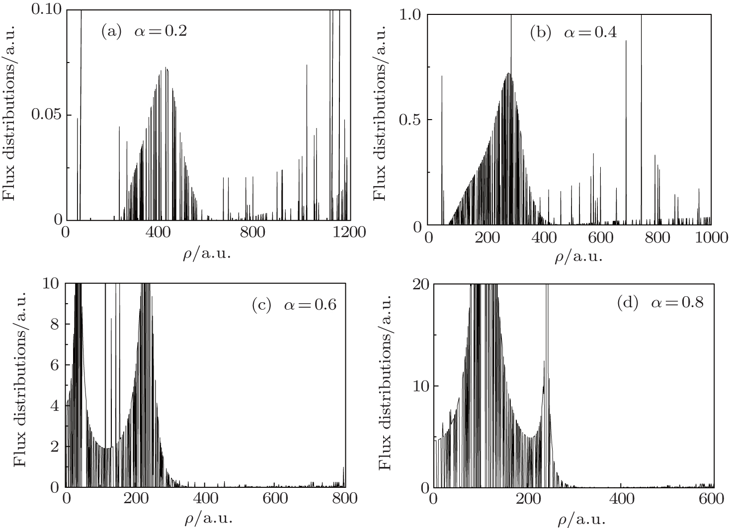 | Fig. 4. Detached-electron flux distributions versus ρ in magnetic field near different dielectric surfaces. The parameters used here are the same as those given in Fig. 3 and the dielectric constant, namely the value of α is given in each diagram. |
Figure 4(a) shows the flux distributions with the value of α being 0.2, there are altogether five boundary points. For 0 < ρ < ρ c1, there are up to ten detached electron trajectories reaching the same position on the detector. For ρ c1 < ρ < ρ c2, there are eight values for θ out corresponding to the same ρ , so there are eight detached electron trajectories reaching the same position on the detector. For any point satisfying ρ c3 < ρ < ρ c4, there are six detached-electron trajectories reaching the same position on the detector, and so on. Under this condition, the maximum impact radius ρ max is about 1200 a.u., so the region of the oscillatory structure in the flux distribution is much more expanded, but the amplitude value of the oscillatory structure in the flux distribution is relatively small. In Fig. 4(b), the value of α increases to 0.4, the number of the boundary points is also five, but the maximum impact radius ρ max decreases to about 1000 a.u., namely the region of the oscillatory structure in the flux distribution decreases and the amplitude value of the oscillatory structure in the flux distribution becomes larger. With the increase of dielectric constant, the number of the boundary points decreases and the maximum impact radius ρ max also decreases.
Figure 3(c) shows the θ out– ρ curve with the value of α = 0.6, there are only two boundary points ρ c1 and ρ c2 . The maximum impact radius ρ max further decreases and the region of the oscillatory structure further decreases also. Because only two orbits interfere on the detector corresponding to the region ρ c1 < ρ < ρ c2, four detached-electron orbits interfere on the detector corresponding to the region 0 < ρ < ρ c1 . Thus the oscillation amplitude in the flux distribution becomes stronger in the range of 0 < ρ < ρ c1 than in the range of ρ c1 < ρ < ρ c2 . With the further increase of the value of α from 0.8 to 1.0, there is only one boundary point and the region of the oscillatory structure in the flux distribution decreases from 605 a.u. to 478 a.u. (see Fig. 4(d)). When the impact radius is in the range of 0 < ρ < ρ c1, there are only two detached-electron orbits reaching the same point on the detector. The flux distribution of detached-electron becomes more oscillatory, and the range of the flux distribution becomes narrow under these conditions. Thus the oscillatory structure in the flux distribution of detached-electron, which is restricted in a small region, becomes much stronger and more obvious.
In order to show the electron flux distribution on the detector surface clearly, we show the two-dimensional contour images of the electron radial probability density distributions (see Fig. 5). It is found that the detached-electron images on the detector consist of bright and dark rings because many classical orbits interfere on the detector. The bright rings correspond to the constructive interference, and the dark rings correspond to destructive interference on the detector. With the increase of the dielectric constant or the value of α increasing from 0.2 to 1.0, the maximum impact radii of the rings become smaller, which shows that the range of detached-electron reaching the detector becomes narrower. So the concentric interference rings become smaller and samller. This result is in excellent agreement with the results given in Fig. 4.
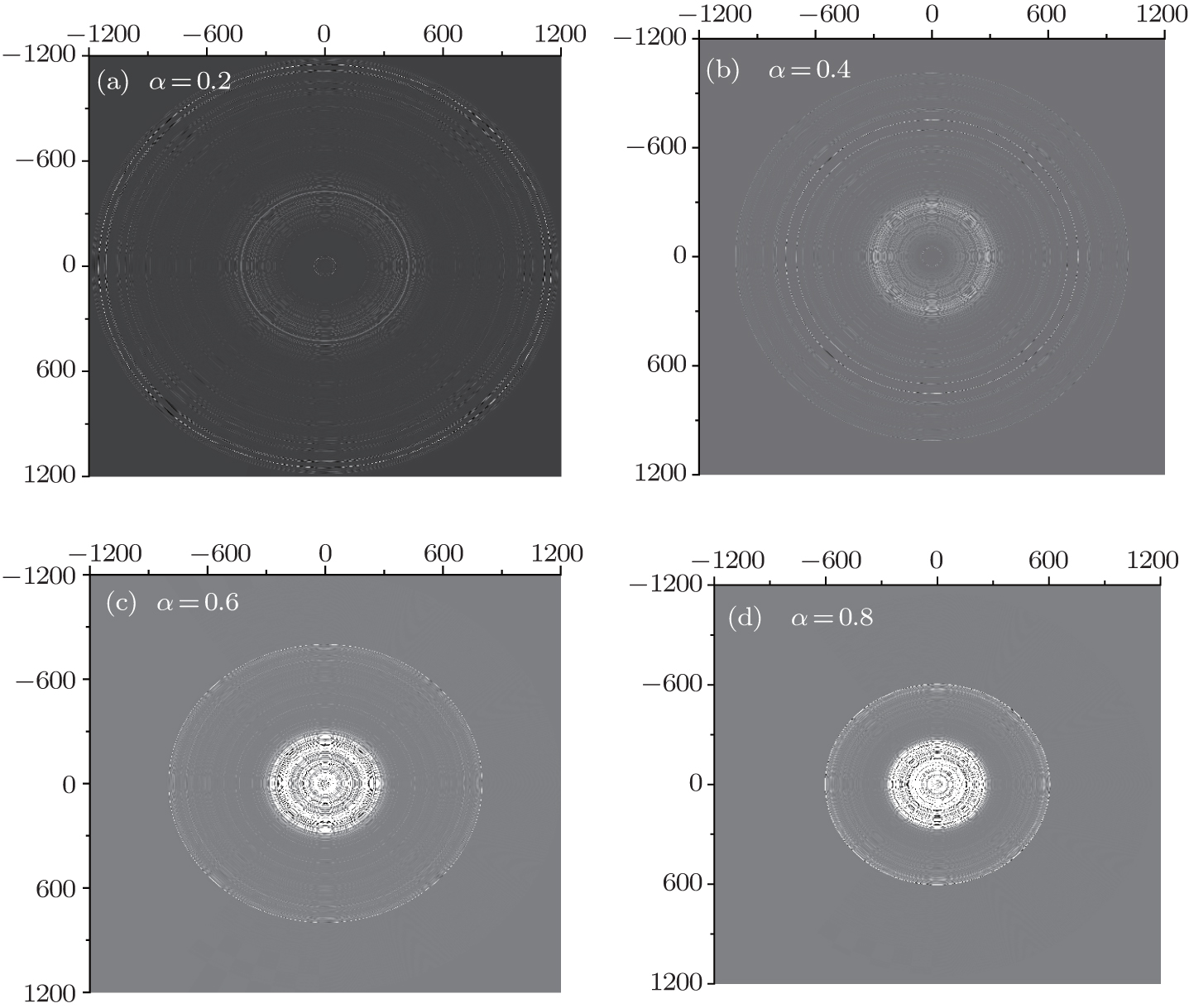 | Fig. 5. Two-dimensional contours of the electron radial probability density distribution for H− in magnetic field near a dielectric surface constant. Detached-electron energy, ion– surface distance, and the position of the detector are the same as those in Fig. 3, the dielectric constants, namely the value of α is given in each image. |
We study the photo-detachment microscopy of H− in the magnetic field near different dielectric surfaces. The semi-classical wave functions for the detached-electron are obtained and the flux distribution on a detector is calculated. The results show that the electron flux distributions of H− are very different in a magnetic field near different dielectric surfaces, namely the dielectric surface has a great influence on the photo-detachment interference pattern of the negative ion. Therefore, the interference pattern in the detached-electron flux distribution can be controlled by using different surfaces. We can see from the two-dimensional contour images the electron radial probability density distribution. To date no experiments on the photo-detachment microscope of H− in the magnetic field near different dielectric surfaces have been carried out. We hope that our results will guide future experimental research on the photo-detachment microscope of the negative ions in the presence of external fields and surfaces.
| 1 |
|
| 2 |
|
| 3 |
|
| 4 |
|
| 5 |
|
| 6 |
|
| 7 |
|
| 8 |
|
| 9 |
|
| 10 |
|
| 11 |
|
| 12 |
|
| 13 |
|
| 14 |
|
| 15 |
|
| 16 |
|
| 17 |
|
| 18 |
|
| 19 |
|
| 20 |
|
| 21 |
|
| 22 |
|