


Theoretical models for designing a 220-GHz folded waveguide backward wave oscillator*
[Cai Jin-Chia), b)†  , Hu Lin-Lin
b) , Ma Guo-Wub) , Chen Hong-Binb) , Jin Xiaob) , Chen Huai-Bia) ]
, Hu Lin-Lin|
|


†Corresponding author. E-mail: caijinchino1@163.com
*Project supported by the Innovative Research Foundation of China Academy of Engineering Physics (Grant No. 426050502-2).
In this paper, the basic equations of beam-wave interaction for designing the 220 GHz folded waveguide (FW) backward wave oscillator (BWO) are described. On the whole, these equations are mainly classified into small signal model (SSM), large signal model (LSM), and simplified small signal model (SSSM). Using these linear and nonlinear one-dimensional (1D) models, the oscillation characteristics of the FW BWO of a given configuration of slow wave structure (SWS) can be calculated by numerical iteration algorithm, which is more time efficient than three-dimensional (3D) particle-in-cell (PIC) simulation. The SSSM expressed by analytical formulas is innovatively derived for determining the initial values of the FW SWS conveniently. The dispersion characteristics of the FW are obtained by equivalent circuit analysis. The space charge effect, the end reflection effect, the lossy wall effect, and the relativistic effect are all considered in our models to offer more accurate results. The design process of the FW BWO tube with output power of watt scale in a frequency range between 215 GHz and 225 GHz based on these 1D models is demonstrated. The 3D PIC method is adopted to verify the theoretical design results, which shows that they are in good agreement with each other.
In recent years, watt-scale, compacted, low cost vacuum electronic device (VED) power source operating between 0.1 THz∼ 1 THz is in urgent demand for the emerging terahertz applications.[1, 2] As a standard seed microwave generator, a 220-GHz backward wave oscillator (BWO) tube is being developed in the Institute of Applied Electronics of China Academy of Engineering Physics (IAE, CAEP). In millimeter or larger wavelength range, the representative slow wave structure (SWS) employed in the BWO tube has a helix structure with pencil beam and inter-digit structures with sheet beam. When the BWO tube is designed to operate in a terahertz regime, the heat conduction ability, machining precision, coupled impedance, system size, and manufacturing cost should all be considered to select a suitable SWS.[3– 9] The folded waveguide (FW) SWS has tremendous advantages due to its planar machining possibilities, all-metal body, moderate coupling impedance, and appropriate dispersion characteristic, thus arousing a hot research interest as SWS in VEDs.[10– 18] The FW BWO has a desirable power-to-volume ratio, great convenience of frequency tunability and relatively low noise, and considerable output power, thereby making it a stable standard seed power source in the terahertz research area.
The design of a 220-GHz FW BWO comprises SWS design, the beam optical system (BOS) design, the power launcher design, and the mechanical design. The basic principle of beam-wave interaction in the BWO tube has been acknowledged by researchers for years.[19– 26] The 3D particle-in-cell (PIC) method is a precise tool to impose a judgment on the design scheme. Nevertheless, it is source-consuming and time-consuming in the preliminary optimization process on the basis of the mainstream computer configuration. The 1D beam-wave interaction equations are then derived in our design stage to give a fast parameter design of the SWS shown in Fig. 1.
 | Fig. 1. Parameters of the FW SWS. |
As a significant part of the 1D model, the axial phase velocity, the interaction impedance and the field attenuation factor of the harmonics of the periodic TE10 mode in the FW SWS are offered in equivalent circuit methods.[12, 13, 27– 31] Through these 1D models introduced here, the parameters of the SWS of the 220-GHz FW BWO are quickly determined for the later mechanical design and design of the BOS. In Section 2, the inherited 1D SSM and LSM are briefly demonstrated. In Section 3, the SSSM specifically for the FW BWO is derived with analytical expressions. In Section 4, the energy distribution of the spent beam analytically derived based on LSM is demonstrated. In Section 5, the design process of the 220-GHz FW BWO based on above models is demonstrated. Finally, some conclusions are drawn from the present study in Section 6.
The 1D frequency-domain beam-wave interaction models for the BWO have been established for years. By substituting for cold wave property values of SWS, the models can be applied to various kinds of BWO tubes. Combined with the equivalent circuit model of FW SWS, the SSM can be used to calculate the start oscillation current and frequency of the FW BWO. Also, the LSM can be adopted to calculate the oscillation frequency and output power when the beam current is larger than the threshold.
The basic equations about the 1D models can be divided into two categories which are like Maxwell equations in their description of interaction on microwave by electron beams and like Lorentz equations in their description of the adverse interaction, respectively.[19– 26] Assuming that the transverse round uniform distribution electron beam passes along the direction of + z axis of the SWS, the synchronized backward space harmonics in the representation of the periodic TE10 mode in the FW should obey the following rule:

where Ezm is the complex amplitude of longitudinal component of the backward harmonics field at z axis, β and α are the phase shift rate and attenuating coefficient of the analyzed backward space harmonic respectively, Kaver is the average coupling impedance of space harmonics in consideration of the round electron beam with a certain diameter, Iz1 is the complex amplitude of the modulated beam current.
The direct current (DC) electron beam will be modulated by synchronized microwave since it moves apart from the entrance of the SWS, denoted as z = 0. By calculating the relationship between the arriving time and the departing time of electrons in a period time of microwave at a certain cross section, the complex amplitude of modulated beam current can be written as follows:

where Iz0 is the direction component of beam current at any position, which equals the emission DC current at z = 0, T is the period time of microwave, and t(t0, z) means the arriving time at z position for the electron particle departing at time t0.
Based on the Lorentz equation, some transformations are conducted to give the following equations:
where η 0 and ve are the absolute values of charge-to-mass ratio and the velocity of the entering electron particles, Ez is the complex amplitude of the whole E-field comprised of space harmonics of periodic TE10 mode and space charge field.
The modulated charged particles can stimulate the space charge field. The alternating component of this field contributes to the whole Ez field. According to the round plate model, the Coulomb method can be used to calculate such a field. The average longitudinal space charge field at a certain z position can be written as follows:[32]

where μ 0n is the n-th positive root of zero-order Bessel function, J means the z component of current density of electron beam at a certain cross section, rm and rc are radii of the electron beam and beam tunnel, respectively. Equation (4) shows that the average space charge field at a certain cross section is relevant to the current density distribution to a total scale. Fortunately, the integration also shows that impact distance is limited to the scale of rc/μ 0n. Around the z position, complex amplitude of modulated current density can be approximated as

With the combination of Eqs. (4) and (5), only the first term of the summation of the series is reserved and the space charge field can be written as

Therefore, the whole Ez field which modulates the beam current can be written as

The power flow can be calculated from the mode field and shown below

The boundary conditions of the FW BWO are determined mainly by the power launcher system, if the discrepancy of mode impedance between periodic TE10 mode in FW SWS and TE10 mode in straight waveguide is ignored, the boundary conditions can be demonstrated as follows:
where Γ 1 and Γ 2 are the voltage reflection coefficients determined by window system and absorber, respectively, Ez* means the corresponding space harmonic E-field of the reversed periodic TE10 mode in FW SWS. In Eq. (8), the reversed mode follows the unperturbed longitudinal evolving principle as a cold wave since it is asynchronous microwave with the electron beam in the general sense.
With the combination of Eqs. (1)– (3), (6), (7), and (9), the backward wave oscillation equations are established. For simplifying the equations into the succinct mathematical expression, some normalizations are conducted as follows:

Notice that Iz0 is a negative number, and C, d, and Q each are a positive number. Therefore, the mathematical model for BWO can be demonstrated by the following equations:

where P0 is the power level of the oscillation mode at entry position. Using this nonlinear model and cold wave properties obtained by equivalent circuit theory, G function is then defined by solving the initial-value problem through the combination of Eq. (11) and Eq. (12), and shown below
where Pe is the DC power of the electron beam, which equals | U0Iz0| ; G function can be calculated through 4-th order Runge– Kutta algorithm given below

The output power and oscillation frequency can be solved by Eq. (14) according to the boundary conditions shown in Eq. (12), when the parameters of the FW SWS and BOS are known.
Equation (14) is a complex equation. This is 1D LSM for the FW BWO concluded from Eqs. (10) and (14).
For the starting oscillation situation where output efficiency | P0/Pe| approaches to zero, t(t0, z) relationship can be written in the following linear perturbation form:

By the combination of Eqs. (11) and (15), the complex amplitude of modulated current can be written in the linear approximation as follows:.

Equation (16) can be written as a differential equation, and shown as follows:

Equations (12) and (17) give the 1D SSM, which are simultaneous linear differential equations. By solving such an initial-value problem, equation (18) is to define function g:


where δ 1, δ 2, and δ 3 are three roots of an algebraic equation, and shown as follows:

Therefore through the linear model and cold wave properties obtained by equivalent circuit theory, the starting oscillation current and starting oscillation frequency can be solved by Eq. (20), when parameters of SWS and BOS are known.

Whether SSM or LSM, iteration algorithm should be adopted to achieve oscillation characteristics of certain backward wave oscillation mode (BWOM). Numerous calculation shows that the equation such as Eqs. (13) and (20) is very sensitive to guessed initial value. Because there are many BWOMs in the FW BWO, it is necessary to put forward a quick method to analytically give estimation about each BWOM, which can also offer the initial value needed in SSM and LSM.
Some approximations should be taken to simplify equations of the SSM. Firstly, periodic TE10 mode in lossy folded waveguide can be seen as the TE10 mode in loss-free straight waveguide, with the consideration of the bended propagation path of microwave. Therefore, the periodic phase shift and mode impedance of TE10 mode can be written as

where a, p, and l0 are defined in Fig. 1, f is the frequency of microwave, c is the light speed in vacuum. According to the definition of space harmonics in equivalent circuit theory, the phase shift rate and coupling impedance at axis can be written as[11, 12]
In the above approximations, the rc and rm are set to be zero equivalently. Here it is assumed that the wave and beam are almost synchronized with each other, the SWS is lossy-free, space charge effect can be ignored, relativistic effect is ignored and end reflection is also disregarded. Hence equation (23) can be derived from Eq. (20) where bC = 0, d = 0, QC = 0, and Γ 1Γ 2 = 0.

By solving Eq. (23), a series of 
For instance, the relations of power flow along z axis of the first four longitudinal BWOMs are shown in Fig. 2.
 | Fig. 2. Power distributions of the first four longitudinal BWOMs. |
The combination of Eqs. (10) and (23) leads to the following equation:

Considering the fact that the BWOM is established by the synchronization of m-order space harmonic with electron beam, the combination of Eqs. (21), (22), and (25) yields the following equation
When specific BWOM marked as TE10n; m is considered, equation (26) actually gives an analytical method to calculate the starting oscillation current and starting oscillation frequency of this specific BWOM. In this denotation of TE10n; m, TE10 means the transverse field distribution, m means synchronized harmonics and n means longitudinal fluctuations of oscillation mode. The solution of the quadratic equation as Φ in Eq. (26) is present in two possibilities: no positive solution tells us that the investigated BWOM cannot be stimulated at all; positive and negative solutions mean that the investigated BWOM can be stimulated with a positive value as a physical solution. The solution process can be explained by intersecting the function curves (see Fig. 3). From Eq. (26) or Fig. 3, the judgment of the existence of TE10n; m can be given as

where N is the periodicity of FW SWS.
 | Fig. 3. Periodic phase shift in starting oscillation situation. In the figure, curve 1 corresponds to π N[1 − (c/ve)· (p/a)], curve 3 corresponds to π N[3 − (c/ve)· (p/a)], curve 5 corresponds to π N[5 − (c/ve)· (p/a)]. |
According to Eq. (14), the power distribution of microwave can be calculated when a certain oscillation mode is established. The other information we are concerned with is the energy spectrum of the electron beam which has interacted with microwave. This is very important for evaluating the interaction efficiency of the BWO and it also gives the initial conditions of entry electron beam for the design of the collector.
The power flow of the electron beam at certain longitudinal position can be calculated by the following equation when the t(t0, z) is primarily calculated:

where E0 is the static energy of electron, which is roughly 511 keV. Generally speaking, the power flow fluctuates with time. The average power flow at a certain position can be derived as

Notice that the entry power of the electron beam is expressed as
The interaction efficiency at a certain position can be calculated from the following equation with the combination of Eqs. (29) and (30)

The maximum and minimum kinetic energy of electron at a certain cross section can be easily expressed as
As for the calculation of energy spectrum of the electron beam, the time period T is divided into N portions to ascertain the contribution of the beam emitting in each time interval. For example, the departing time points

are considered, which is a natural numerical truncation to realize LSM. The kinetic energy of a certain electron departing at ti when it arrives at the cross section at the position of z can be expressed as
Therefore, the electron departing between ti and ti+ 1 will contribute to probability density by | Ei+ 1 − Ei| − 1M− 1. The energy spectrum can be obtained by summing up operations, and demonstrated as
Using SSSM, the starting oscillation frequency and current of BWOMs in the FW BWO can be calculated very fast. The initial parameters of SWS and beam optical system are optimized in Table 1.
| Table 1. Parameters for calculating the starting oscillation. |
The SSSM shows that the operating mode TE100; − 2 has a starting oscillation current of 2.05 mA and starting oscillation frequency of 220.36 GHz. The SSSM also shows that the second BWOM is TE100; − 3 which possesses a starting oscillation current of 7.82 mA and frequency of 304.00 GHz, and the third BWOM is TE101; − 2 which possesses a starting oscillation current of 13.70 mA and frequency of 219.13 GHz.
Using small signal model (SSM) and equivalent circuit theory, the FW BWO with parameters as shown in Table 1 is verified and optimized further. The most additive factor which has a great influence on starting oscillation current is the radii of beam tunnel and electron beam. With the compromise of the larger coupling impedance and more relaxed machining and assembly error tolerance, the filling factor of the electron beam is roughly set to be 0.8. The next point to be reckoned on is the emission current density. Since the mature M-coated thermionic cathode with a maximal emission current density of just 5 A/cm2 will be used to generate the electron beam, the DC threshold current density of the electron beam in the beam tunnel should be optimized to be as little as possible to ease the cathode burden by sweeping the value of rc. The effective conductivity of copper is roughly set to be 1.8× 10⁷ Ω − 1· m− 1 by analytical method, [33] which shows more Ohmic losses than that in a real situation to give a conservative prediction. Both in SSSM and SSM, the end reflection is ignored.
The SSM shows that the operating mode TE100; − 2 has a starting oscillation current of 11.82 mA and starting oscillation frequency of 221.80 GHz. The SSM also shows that the second BWOM is TE101; − 2 which possesses a starting oscillation current of 427.41 mA and starting oscillation frequency of 219.74 GHz and the third BWOM is TE100; − 3 which possesses a starting oscillation current of 471.39 mA and starting oscillation frequency of 302.44 GHz. Apparently, the mode competition problem can be ignored when the operating current is several times as large as the threshold current.
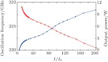
When the operating current is higher than the threshold current, the oscillation frequency and output power can be calculated by LSM, which are shown in Fig. 4.
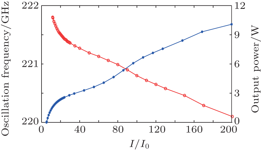 | Fig. 4. Variations of oscillation frequency and output power with beam current. |
The output power increases drastically when the beam current exceeds the threshold and then increases steadily as the beam current further grows. In time domain analysis, the transient process shows that the over-bunch instability occurs when I/I0 is larger than 3∼ 4 in general, [21, 34] which is also checked by later PIC simulation. On the other hand, the emission ability of the accessible cathode should be taken into consideration. Therefore, the operating current is determined to be 22 mA and the voltage is also adjusted to 15.0 kV to make the oscillation frequency approximate to 220 GHz.
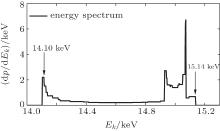
With these parameters, the LSM demonstrates that the FW BWO can generate microwave with an output power of 1.98 W at a frequency of 220.05 GHz. The peak power happens at the third entry of the SWS, which is about 1.5 times the output power. This phenomenon is caused by ohm loss of the FW SWS. The efficiency of the FW BWO can then be calculated to be 0.6%. The interaction efficiency calculated by Eq. (31) is roughly 1.9%. The energy spread is from 14.10 keV to 15.14 keV, which is shown in Fig. 5. The relatively low efficiency is caused by large ohm loss and low electron beam current, which is always a technical bottleneck in the development of THz VEDs.
 | Fig. 5. Energy spectrum of spent beam. |
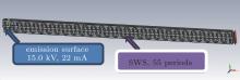
The PIC method is used to verify our theoretical design of the FW BWO. A 3D computer code is employed to give a convincing comparison. The PIC model is established as shown in Fig. 6, where a uniform axial magnetic field is set to be 50 times the Brillouin field to mock the 1D movement of the electron beam. The numerical results of the PIC simulation are shown in Fig. 7, after mesh convergence analysis has sufficiently been conducted. The results show great consistency with our 1D theoretical model, where less than 1% error occurs.
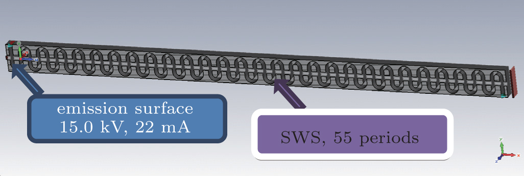 | Fig. 6. PIC model of folded waveguide BWO. |
 | Fig. 7. Numerical results of 3D PIC simulation. |
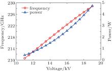
The backward wave oscillation is finally stabilized after 10 ns∼ 20 ns. In consideration of the model errors of 1D theoretical method, the beam voltage and beam current are finally determined to be 15.4 kV and 22 mA to make the oscillation frequency stay at 220 GHz according to further PIC simulation. As a BWO, the voltage tuning frequency bandwidth is also estimated by LSM, which is shown in Fig. 8. The current varies with voltage according to the 3/2 power law which has been regarded as a space charge principle since the convergence Pierce gun was launched.[35] In our required frequency range between 215 GHz and 225 GHz, the output power remains watt scale.
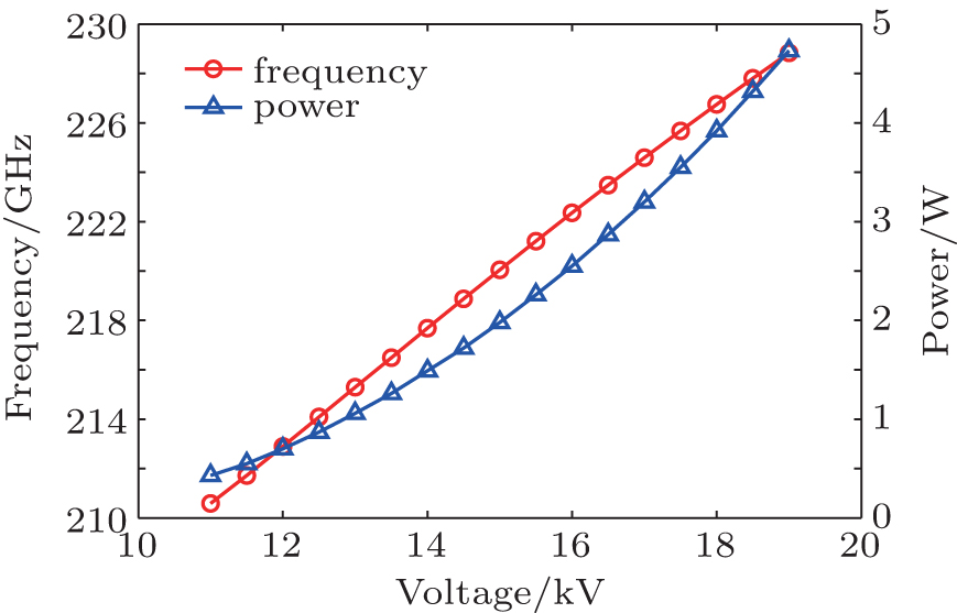 | Fig. 8. Tunable bandwidth estimated by LSM model. |
The consuming CPU times of SSSM, SSM, LSM, and PIC method in a present mainstream computer with a dominant frequency of 3 GHz and a RAM of 8 GB are several microseconds, seconds, minutes, and days, respectively. The model accuracy is enhanced one-by-one whereas the results of a rougher model can offer a reference to the following, more accurate model. Based on this model, the parameters of SWS and BOS are determined and the design process is time-saving and more efficient than the parameter sweep purely based on 3D PIC simulation.
An FW BWO is finally designed in this paper, with watt-scale output in a frequency range between 215 GHz and 225 GHz. The theoretical models introduced here can be naturally extended to more FW BWO tubes in other microwave frequency bands.
The window system and the beam optical system have already been designed and tested.[36, 37] The whole prototype tube is under machining.
| 1 |
|
| 2 |
|
| 3 |
|
| 4 |
|
| 5 |
|
| 6 |
|
| 7 |
|
| 8 |
|
| 9 |
|
| 10 |
|
| 11 | [Cited within:1] |
| 12 |
|
| 13 |
|
| 14 |
|
| 15 |
|
| 16 |
|
| 17 |
|
| 18 |
|
| 19 |
|
| 20 |
|
| 21 |
|
| 22 |
|
| 23 |
|
| 24 |
|
| 25 |
|
| 26 |
|
| 27 |
|
| 28 |
|
| 29 |
|
| 30 |
|
| 31 |
|
| 32 |
|
| 33 |
|
| 34 |
|
| 35 |
|
| 36 |
|
| 37 |
|