Fractional-order systems have become an active research field in recent years. Since the fractional calculus enables us to describe real world physical phenomena more accurately than the classical integer calculus, the research on the dynamics, control, and applications of fractional-order systems deserves considerable attention.^{[1, 2]} The controls of linear and nonlinear systems have been reported in a lot of literature related to the system stability analysis, ^{[3– 6]} controller design, ^{[7, 8]} system simulation, etc. Among many physical and biological fractional-order systems, it has been confirmed theoretically and practically that the chaotic behaviors exist in the fractional-order systems, such as fractional-order Chua’ s system, ^[9] fractional-order financial system, ^[10] and fractional-order unified chaotic system, ^[11] etc.

Synchronization of fractional-order chaotic systems is of significance for real world physical applications. Fractional-order chaotic systems have been found in physics, engineering, finance, and sociology. The control and synchronization of fractional-order chaotic systems have been used successfully in many real applications, such as permanent magnet synchronous motor, ^[12] circuit design, ^[13] and secret communication.^[14] For classical chaotic system synchronization, much research work has been done in some areas, such as linear control, ^[15] nonlinear state feedback control, robust control, ^{[16, 17]} and sliding mode control.^{[18– 20]} In recent years, control research on the synchronization of fractional-order chaotic systems were extensively investigated.^{[21– 25]} However, the integer-order stability analysis tools are inapplicable for fractional-order chaotic systems in the sense of Lyapunov stability.

For fractional-order nonlinear stability analysis, the generalized Mittag– Leffler stability^[26] is a powerful tool, in terms of fractional Lyapunov function, to prove controlled system stability. Although an appropriate candidate Lyapunov function is often hard to obtain, some recent work^{[27, 28]} provides suitable fractional-order inequalities and analysis techniques to facilitate the process of controller design.

To our best knowledge, the work on the synchronization of fractional-order chaotic systems with uncertain parameters, model uncertainty or additive disturbance, is not so much in the sense of the generalized Mittag– Leffler stability. In practical applications, it is inevitable to encounter the situation where systems are often with various uncertainties, ^{[29, 30]} which will be considered in this paper.

In our contributions, we use the generalized Mittag– Leffler stability to deal with the synchronization of fractional-order chaotic systems with uncertain parameters and uncertain disturbances. To our best knowledge, most of the studies are based on traditional Lyapunov stability, however we employ the generalized Mittag– Leffler stability, which implies Lyapunov asymptotic stability, to design the controller, by constructing a fractional Lyapunov function. The uncertainties are often caused by model uncertainty and additive noise, and these uncertainties usually can be dealt with under certain conditions that the uncertainties are assumed to be bounded either by a known or an unknown constant. For the case that uncertainties are bounded by a known constant, a robust or adaptive control proposed in the cited references in this paper can be employed to deal with this situation. Meanwhile, for the case of an unknown constant, limited work has addressed this issue before and we propose fractional-order update laws for the unknown parameters and unknown upper bounds of the uncertainties respectively. An adaptive control combined with fractional-order state feedback and uncertainty estimates is proposed to synchronize two fractional-order chaotic systems. Although the proposed control law consists of multi-controllers, it presents a new insight into this issue theoretically and it holds true for most of the chaotic systems, even the synchronization between two different chaotic systems as will be discussed later in Corollary 2. Finally, illustrative examples and simulations are provided to demonstrate our control design.

The rest of this paper is organized as follows. In Section 2, fractional calculus properties and fractional-order system stability criteria are introduced. In Section 3, the adaptive control design and estimated update laws are presented. In Section 4, illustrative examples and numerical simulation results are provided. Finally, some conclusions are drawn from the present studies in Section 5.

Definition 1 Let f : [a, b] → R and f ∈ L¹[a, b]. The Caputo fractional derivative of order α is defined as

where α ∈ R⁺ and Γ (· ) is the Gamma function. The order of the chaotic system is 0 < α < 1. In this paper we employ D for representing the classical integer differential D¹f (t) = d f (t)/dt.

Furthermore, there are some properties for the fractional calculus.^[10]

(i) For α = n, where n is an integer, the fractional-order derivative coincides with the integer order derivative. Particularly, when α = 0, it appears as the identity operator, i.e.,

(ii) The fractional operator is a linear operator

where a and b are real constants.

Theorem 1^[26] Let x(t) = 0 be the equilibrium point of the fractional-order system D^α x = f (x, t), x ∈ D ⊂ Rⁿ, where D contains the origin. Assume that a fractional Lyapunov function V(x, t) : Rⁿ × [0, ∞ ) → R is a continuous differential function and locally Lipschitz with respect to x, and there exists class-K function γ _i such that

then x(t) = 0 is asymptotically stable. Moreover, if the conditions hold globally on D = Rⁿ, then x(t) = 0 is globally asymptotically stable.

The above theorem deals with system stability in the sense of fractional order, and is also called the generalized Mittag– Leffler stability theorem. It should be noted that Mittag– Leffler stability implies Lyapunov asymptotic stability.^[26]

Theorem 2^[5] Let fractional-order linear time-invariant (LTI) system D^α x(t) = Ax(t), where A ∈ R^{n× n} and x ∈ Rⁿ, if the following condition is satisfied:

then the LTI system is asymptotically stable.

Since the fractional Lyapunov function described in Theorem 1 must work within the framework of fractional-order inequalities, here we present some powerful inequalities concerning the fractional-order systems.

Lemma 1^[27] Let x(t) ∈ R be a continuous and derivable function, then, for any time t ≥ 0, the following inequality will always hold:

where α ∈ (0, 1).

Lemma 2^[28] Let x(t) = [x₁(t), … , x_n(t)] ∈ Rⁿ be a real-valued continuous and derivable vector function, then, for any time t ≥ 0, the following inequality will always hold:

where α ∈ (0, 1) and P = diag[p₁, … , p_n] > 0.

Remark 1 The above two lemmas are conducive to constructing fractional Lyapunov candidate function through transforming the well-used quadratic function in Lyapunov direct method into system fractional differential equations by inequality.

Consider a pair of fractional-order uncertain chaotic systems. The drive system can be described by

The response system with unknown uncertainties can be described by

where the system state x ∈ Rⁿ, y ∈ Rⁿ, and α ∈ (0, 1) is the order of the fractional derivative; f_i and (i = 1, … , n) are continuous nonlinear system vector functions; θ _i ∈ R^m_i (i = 1, … , n) are the unknown parameters in the drive system; ∊ R^m_i (i = 1, … , n) are the estimates of θ _i in the drive system; Δ f_i(y, t) (i = 1, … , n) are unknown model uncertainty terms; d_i(t) (i = 1, … , n) are external disturbances of the system; u_i (i = 1, … , n) are system controllers.

The system error is defined as e = y − x, and systems (8) and (9) are said to be synchronized under arbitrary initial conditions x(0) and y(0) if

The error system can be represented by the following equations:

where and Δ f_ei = Δ f_i(y, t) + d_i(t).

Assumption 1 The unknown model uncertain terms Δ f_i(y, t) and external disturbances d_i(t) are all bounded by unknown positive constants, which implies

where δ _i (i = 1, … , n) are unknown positive constants.

Remark 2 The term Δ f_ei is introduced for simplifying the system expression, and one can also consider Δ f_i (y, t) and d_i(t) directly instead of Δ f_ei, which makes no difference in the error system asymptotic stability. Furthermore, it is also available to consider uncertain terms and external disturbances in the drive system  (8), and this consideration only leads to the change of Δ f_ei. It can be seen that our control method is valid under the Assumption  1, thus it will also work if the uncertainties are considered in both drive system and response system.

Theorem 3 The error system (11) with uncertainties can be globally stabilized asymptotically by the adaptive feedback control

where s_i = e_i + λ _iD^{− α} e_i,

λ _i and k_i are constants, update laws

and

with being the estimate of the unknown parameter θ _i, and being the estimate of the unknown upper bound δ _i in Assumption 1; Γ _i = diag[p_i1, … , p_im] > 0 and r_i > 0 are the gains of the update laws respectively.

Proof The procedure of the proof consists of two steps.

Step 1 By introducing s_i = e_i + λ _iD^{− α} e_i for the i-th equation in error system (11), and using the Caputo derivative, we obtain

Choosing Lyapunov function for the i-th equation

where is the parameter estimate error and is the upper bound estimate error, using the Caputo derivative, and according to Lemma  1 and Lemma  2 we have

By Eq.  (16), we have

Substitute control u_i and note that

we have

By use of update laws  (14) and (15) and noting that we have

Step 2 Choose Lyapunov function for the whole error system  (11), then we have

If D^α V = 0, which implies s_i = 0, thus the error system becomes

By choosing λ _i appropriately to satisfy Theorem  2, the error system achieves asymptotic stability.

If D^α V < 0, and since is positive-definite, based on the relationship between class-K functions and positive-definite functions, there exists a class-K function γ such that D^α V ≤ − γ (‖ η ‖ ), where . According to Theorem  1, the error system is asymptotically stable. This completes the proof.

Corollary 1 Theorem 3 makes it also possible to design a simpler feedback control in the way of replacing s_i by e_i. In this case, the items k_isgn(s_i) and m_i in u_i become k_ie_i and

respectively. Follow the two steps in the proof, we have

and

If D^α V = 0, this implies e_i = 0; otherwise D^α V < 0, thus the error system is asymptotically stable according to Theorem  1.

Corollary 2 It is also available to achieve the synchronization of two different fractional-order chaotic systems, based on Theorem 3. In this case, the response system (9) becomes D^α y_i(t) = g_i(y) + Δ f_i(y, t) + d_i(t) + u_i and f_ei(e) = g_i(y) − f_i(x) in the error system  (11) correspondingly. Following the procedure of the proof of Theorem 3, we can design an adaptive control for the synchronization between two different chaotic systems, which case will be illustrated in Example 3 in the simulations.

In this section, we will give numerical simulations to illustrate the effectiveness of the proposed adaptive control.

Example 1 Consider the fractional-order Van der Pol oscillator

where α ∈ (0, 1) and ε is the system parameter. The response system within unknown ε is expressed as

the adaptive control is

and the update laws are

Figures  1 and 2 show the convergence of the Van der Pol error system and the system synchronization, with initial conditions x(0) = [2, − 3]^⊤ , y(0) = [5, 4]^⊤ , gains of update law p = 1, r_i = 2, model uncertainties Δ f_i = 0.5cos(π t), external disturbances d_i(t) = 0.1sin(5t); control parameters k_i = 2 and λ _i = 1; system order α = 0.96.

Fig.  1.

	Figure Option ViewDownloadNew Window
	Fig.  1. Convergence of Van der Pol error system.

Fig.  2.

	Figure Option ViewDownloadNew Window
	Fig.  2. Synchronization of Van der Pol systems.

Example 2 Consider the fractional-order Genesio– Tesi system

where α ∈ (0, 1) and β _i are the system parameters. The response system with unknown β ₁ and β ₂ is expressed as

the adaptive control is

and the update laws are

Figures  3 and 4 show the convergence of the Genesio– Tesi error system and the system synchronization, with initial conditions x(0) = [0.1, 0.5, − 0.2]^⊤ , y(0) = [− 1, − 2, 1]^⊤ , and gains of update law p_i = 2, r_i = 3; model uncertainties Δ f_i = 0.4sin(π t); external disturbances d_i(t) = 0.2cos(5t); control parameters k_i = 1 and λ _i = 3; system order α = 0.98.

Fig.  3.

	Figure Option ViewDownloadNew Window
	Fig.  3. Convergence of Genesio– Tesi error system.

Example 3 Consider the synchronization of two different chaotic systems as discussed in Corollary 2. The drive system is the Lorenz system

where α ∈ (0, 1); a and c are the unknown parameters. The response system is chosen to be the Lü system with uncertainties

where α ∈ (0, 1); τ , ρ , and β are the system parameters. The adaptive control is

and the update laws are

Fig.  4.

	Figure Option ViewDownloadNew Window
	Fig.  4. Synchronization of Genesio– Tesi systems.

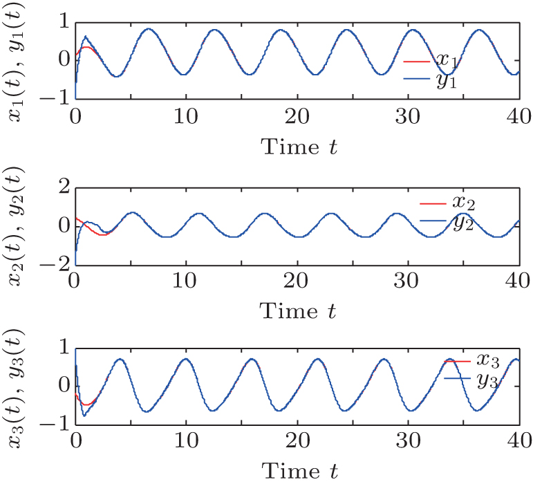
Figures  5 and 6 show the convergence of the errors and the synchronization between two different chaotic systems, with initial conditions x(0) = [0.1, 0.1, 0.1]^⊤ , y(0) = [6, − 6, 5]^⊤ , β = 20, ρ = 3, τ = 36, b = 1, ĉ (0) = 3, and â (0) = 9; gains of update law p_i = 6, r_i = 4; model uncertainties Δ f_i = 0.2sin(π t); external disturbances d_i(t) = 0.1cos(8t); control parameters k_i = 3 and λ _i = 3; system order α = 0.98.

Fig.  5.

	Figure Option ViewDownloadNew Window
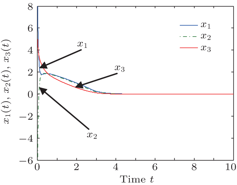	Fig.  5. Convergence of errors between Lorenz and Lü systems.

Fig.  6.

	Figure Option ViewDownloadNew Window
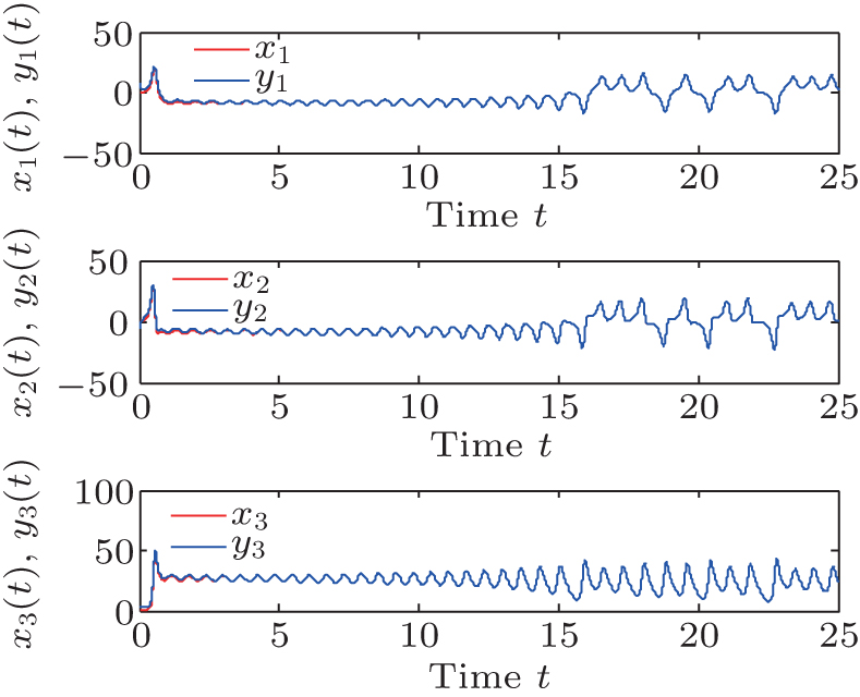	Fig.  6. Synchronization between Lorenz and Lü systems.

From Fig.  1 to Fig.  6, it is obvious that Van der Pol oscillator system, Genesio– Tesi system and Lorenz system are well synchronized by the adaptive control proposed in this paper. Based on the comparison of the three examples in the simulations, it is concluded that both the control parameters and the gains of update laws have influences on the convergence speed. When increasing the control parameters and update law gains, the error systems converge faster. Furthermore, when fractional orders of the systems increase, the error systems converge faster. The system unknown parameters, model uncertainties, and external disturbances can be well dealt with under arbitrary initial conditions, which confirms the effectiveness of our control method.

In this paper, we consider the synchronization of two fractional-order chaotic systems with unknown parameters and uncertainties. Based on fractional Lyapunov function, an adaptive control combined with the fractional-order nonlinear state feedback and estimated update laws is proposed to stabilize the fractional-order error system with asymptotic convergence. The unknown parameters and unknown uncertainties can be well dealt with under fractional order the update laws of the proposed controller. Illustrative examples and simulation results are provided to demonstrate our control scheme.