There are several paradigmatic three-dimensional chaotic flows. Aside from the ubiquitous Lorenz and Rö ssler systems, one of the most intricate and widely studied systems is Chen’ s system, proposed in 1999.^[1] Each of these systems represents a topological distinct genus of chaos. In 2002 Aziz-Alaoui and Chen^[2] presented a piecewise linear Chen system modeled by the following initial value problem (IVP)

with x₀ ∈ ℝ ³, T > 0, a, b, c, d some positive real parameters verifying the condition a < c.

While the genuine Chen system^[1] is a continuous system, having the following mathematical model

(with a = 35, b = 3, and c = 28), the system (1) is a piecewise linear (PWL) system. The detailed asymptotic analysis of this system, including a study of the chaotic behavior with the bifurcation parameter, is presented in Ref. [2].

Fractional calculus has been a topic for more than 300 years, but recently, systems of fractional-order have attracted much attention after the first numerical methods have been performed. Fractional-order systems play an important role in many fields of science and engineering (see e.g. Refs. [3]– [11] or Refs. [12] and [13] with therein references). Also, piecewise continuous functions are used in the study of nonlinear circuits and systems. They are also commonly employed in the modeling of the memristor, leading to many novel studies and applications (see e.g. Refs. [14]– [16]).

Motivated by the huge interest in Chen’ s system of integers and fractional-order (see e.g. Refs. [1] and [17]), we present in this paper a new and more general extension of the PWL system (1): the PWL Chen system of fractional-order, modeled by the following differential equations

with a = 1.15, b = 0.15, c = 2, and d = 0.1.

(for q = (q₁, q₂, q₃)) stands for Caputo’ s differential operator of order q with starting point 0 (see e.g. Refs. [18]– [20]). Recall that the Caputo differential operator is a fractional extension of differentiation defined for n − 1 < q ≤ n, q ∈ (0, ∞ )\ℕ , n being some positive integer, defined as follows:

where Γ is Euler’ s function.

In contrast to alternative definitions of fractional differentiation, Caputo’ s derivative gives a physical interpretation to the included initial conditions, necessary in practical problems.^{[21, 22]} Using this definition, one avoids the expression of initial conditions with fractional derivatives and therefore the initial condition can be considered in the standard form x(0) = x₀.

As in the most practical examples, in this paper we consider q_i ≤ 1, i = 1, 2, 3.

The chaotic behavior of PWL Chen’ s system (3) as a function of the commensurate order q is revealed by the bifurcation diagram (BD) in Fig. 1(a)¹⁾. A few representative attractors are plotted in Figs. 1(b)– 1(e). As is well known, for systems of commensurate order, chaos persists over a minimal commensurate order q_min < 1, i.e., a system order 3 × q_min < 3. Revealed numerically by the BD, q_min for our system is about 0.865, which indicates that chaos exists for a system order greater than 3 × q_min = 2.575 (compare with the continuous Chen’ s system of fractional-order^{[12, 17]}).

Fig. 1.

	Figure Option ViewDownloadNew Window
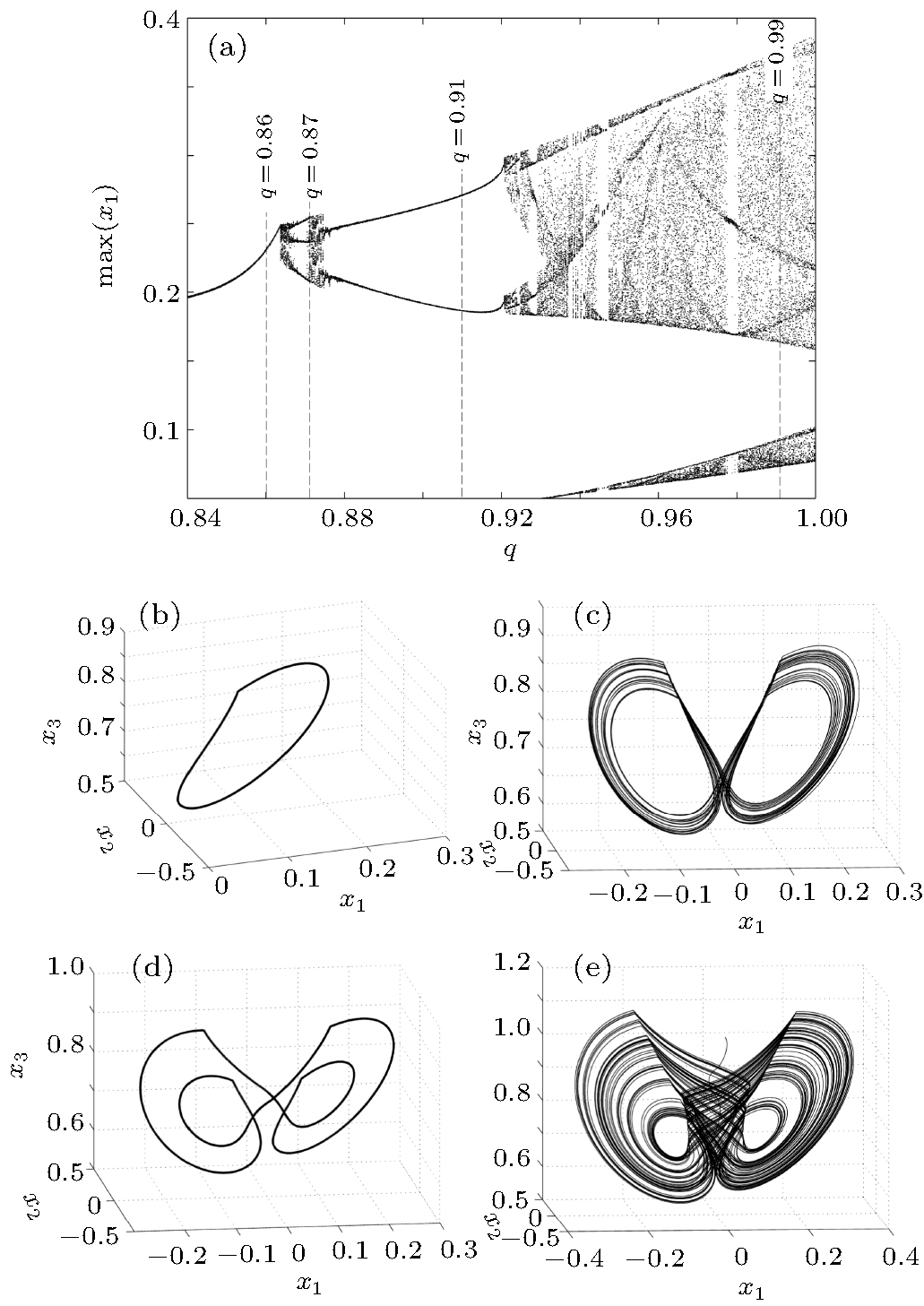	Fig. 1. Bifurcation diagram of Chen’ s system (3) for the commensurate fractional-order q ∈ [0.84, 1]; (a)– (e) Attractors corresponding to q = 0.86, q = 0.87, q = 0.91, and q = 0.99 respectively.

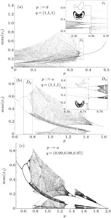
Let us denote by p the single scalar bifurcation parameter, which for the considered system (3) can be any of the four parameters a, b, c or d. Two representative cases have been considered here: p : = d, integer case q = (1, 1, 1), and p: = a, integer case q = (1, 1, 1), and the incommensurate fractional-order case q = (0.99, 0.98, 0.97). For the sake of conciseness we do not present results of computation here, but we have found that the other two cases (p : = b and p : = c) demonstrate a similar behavior. We find particularly rich bifurcation behaviors, revealed by the BDs in Fig. 2. The results are for: (a) p : = d in the integer-order case, with a = 1.15; (b) p : = a in the integer order case; and (c) for p : = a with the fractional-order case.

Fig. 2.

	Figure Option ViewDownloadNew Window
	Fig. 2. Bifurcation diagrams of Chen’ s system (3); (a) p : = d, q = (1, 1, 1) and a = 1.15, c = 2 and b = 0.15; (b) p : = a, q = (1, 1, 1) and b = 0.15, c = 2 and d = 0.1; (c) p = a, q = (0.99, 0.98, 0.97) and b = 0.15, c = 2 and d = 0.1.

It is easy to verify that, in addition to the origin, the system has two equilibrium points

(see Table 1). Because the equilibrium points reside in the plan x₁ = x₂, and are not equilibrium points for this system (see Ref. [1]). The coordinates present symmetries which are also evident in the simulations of the state variables x₁ and x₂. These symmetries come from the invariance of the vector field under rotation symmetry (x, y, z) → (− x, − y, z). To note that for the chosen values of parameters a, b, c, and d, with a < c, the state coordinate is positive while can be either positive and negative.

Table 1.

Table 1.

Table 1. Equilibrium points of the PWL Chen system (3).

Table 1. Equilibrium points of the PWL Chen system (3).

As can be seen from the detail in Figs. 2(a) and 2(b), for p : = d and p : = a respectively, a new characteristic has been uncovered for this system, the multistability, i.e., the coexistence of regular and chaotic motions in some parameter windows (details D₁ in Fig. 2(a) and D₂ in Fig. 2(b)). Therefore, for a specific value p in these windows, depending on the basin of attraction and initial conditions, we can find coexisting attractors. For example, for a = 1.15, b = 0.15, c = 0.1, and with p : = d = 0.361 chosen in the window [0.345, 0.370], we found two different attractors: a chaotic one and a stable cycle (see D₁ in Fig. 2(a)). For b = 0.15, c = 2, d : = 0.1 and with p : = a chosen in the window p ∈ [0.7, 0.8], the two attractors are plotted in detail D₂ in Fig. 2(b).

In the remainder of this paper we show numerically, aided by computer simulations, that every stable attractor of Chen’ s system (3) can be numerically approximated by a Parameter Switching (PS) algorithm.^[23] The PS algorithm switches p within a chosen set, while the IVP is numerically integrated with some numerical scheme with fixed step size. The convergence of the PS algorithm to some desired attractor is presented in Refs. [24] and [25].

The paper is structured as follows: in Section 2, the PS algorithm is explained, Section 3 presents the continuous approximation of the IVP (3) and in Section 4 several stable attractors of the PWL Chen system of fractional-order are approximated with the PS algorithm.

Let a continuous system of fractional-order be modeled by the following IVP

where: A ∈ ℝ ^{n× n} is a real square constant matrix; f : ℝ ⁿ → ℝ ⁿ is a nonlinear, at least continuous function and q ≤ 1. The great majority of known systems of integer or fractional-order, including systems like: Lorenz, Chen, Rö ssler, Chua, Rikitake, and many other systems, are modeled by the IVP (4). In Refs. [24] and [25] it was proved analytically and verified numerically that the PS algorithm allows the numerical approximation of any desired attractor, by switching the control parameter within a chosen finite set of values while the underlying IVP is numerically integrated with some fixed step-size numerical method.

Next, assume that the IVP enjoys the uniqueness Lipschitz continuity which is a common sufficient condition for both integer and fractional case (see Ref. [26] Corollary 6.9 for FDE uniqueness). Furthermore, denote by 𝒫 _N = {p₁, p₂, … , p_N}⊂ ℝ , N ≥ 2, the switching values set.

Remark 1 Due to the uniqueness assumption, it is reasonable to consider that to each p_i ∈ 𝒫 _N, i ∈ {1, 2, ..., n}, it corresponds to a unique attractor A_pi. As usual for numerical tests, in this paper we consider the attractors as being the trajectory of the underlying numerical solution, after sufficiently long transients are removed.

By choosing 𝒫 _N, while the underlying IVP is numerically integrated with a fixed step-size h, PS switches in some deterministic (periodic) way the control parameter within 𝒫 _N, for relatively short time subintervals. The obtained “ switched solution” will approximate the “ averaged solution” obtained for p replaced with the average of switched values. Following Remark 1, the attractor corresponding to the switched solution, will approximate as closely as desired (depending on the numerical integration accuracy limitation), the attractor corresponding to the averaged solution. The numerical integrations have been realized with the standard Runge– Kutta (RK4) method for the integer-order case and the Adams– Bashforth– Moulton (ABM) method^[22] for the fractional-order case (see also Ref. [27]).

Schematically, for a chosen set 𝒫 _N with the “ weights” set ℳ = {m₁, m₂, ..., m_N}, and a fixed step-size h, the way in which PS algorithm works can be expressed schematically as follows:

The scheme (5) means that for the first m₁ integration steps the control parameter p will take the value p₁, then, for the next m₂ integration steps, p = p₂, and so on until, for m_N times, p = p_N, after which, again p = p₁ for m₁ times, then p = p₂ for m₂ times and so on until the considered time integration interval, [0, T], is covered. For example [2p₁, p₂] means that while the IVP is integrated, p will take the values: p = p₁, p = p₁, p = p₂, p = p₁, p = p₁, p = p₂, and so on.

Let us denote the “ weighted average” of the values of 𝒫 _N by

Then, the “ switched attractor” , A*, obtained with the PS algorithm, will approximate the “ averaged attractor” , A_p*, obtained by integration of the underlying IVP with p replaced with p*. The analytical proof of the convergence, for the integer-order case, is presented in Refs. [24] and [25], while for fractional-order systems the convergence has been computationally verified for several systems (see e.g. Ref. [23]).

Remark 2 The PS algorithm can be used both as a control and an anticontrol-like technique when, by some objective reasons, some certain targeted parameter value p* cannot be accessed directly. In this case, we have to select the set 𝒫 _N, m_i, i = 1, 2, … , N and an adequate scheme (5) to obtain, with Eq. (6), the targeted value p*. For example, if the values of 𝒫 _N generate chaotic behavior and p* generates a regular motion, the PS algorithm acts like a control-like algorithm. However, while most known control/anticontrol algorithms “ force” the trajectory to change its characteristics and behavior, the PS algorithm allows us to obtain approximation of any desired existing attractor.

Also, the PS algorithm can help to enrich our understanding of what happens in some real systems when the control parameter is switched by natural causes.

Finally, the PS algorithm proves that p switchings present a robustness-like property in the following sense: for whatever sets 𝒫 _N, ℳ , if p_min = min{𝒫 _N} and p_max = max{𝒫 _N}, the obtained values p* remains between p_min and p_max. Note that the PS algorithm applies also for discrete-time real systems and some interesting results have been obtained for complex discrete-time systems, ^[25] although that is beyond what we consider in this paper.

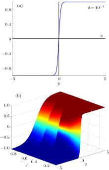
The main obstacle in applying the PS algorithm to PWL systems is the lack of numerical methods specifically devised for fractional differential equations with discontinuous right-hand side (Filippov-like systems of fractional-order). This is one of the reasons that discontinuous systems of fractional-order have been not rigorously studied. One possible approach to surpass the obstacle of integration of discontinuous differential equations of fractional-order, is to approximate continuously the underlying discontinuous IVP, based on the transformation of the IVP into a set-valued one, which next can be continuously approximated with a single-value IVP (see Ref. [28]). Thus, piecewise constant components, like sgn, can be continuously approximated globally (in small neighborhoods of the graph) or locally (in a small neighborhood centered at the discontinuity point x = 0). In this paper we use the global sigmoid approximation

which approximates globally the sgn function, on small neighborhoods of its graph. In Fig. 2(a), for clarity, δ has been chosen to be larger (δ = 10^{− 1}), while in Fig. 3(b), sgn is drawn as a function of two variables: x and δ . The parameter δ controls the slope of the sigmoid function, near the discontinuity x = 0. As proved in Ref. [28], for numerical purposes an adequate choice is δ = 10^{− 5}.

Fig. 3.

	Figure Option ViewDownloadNew Window
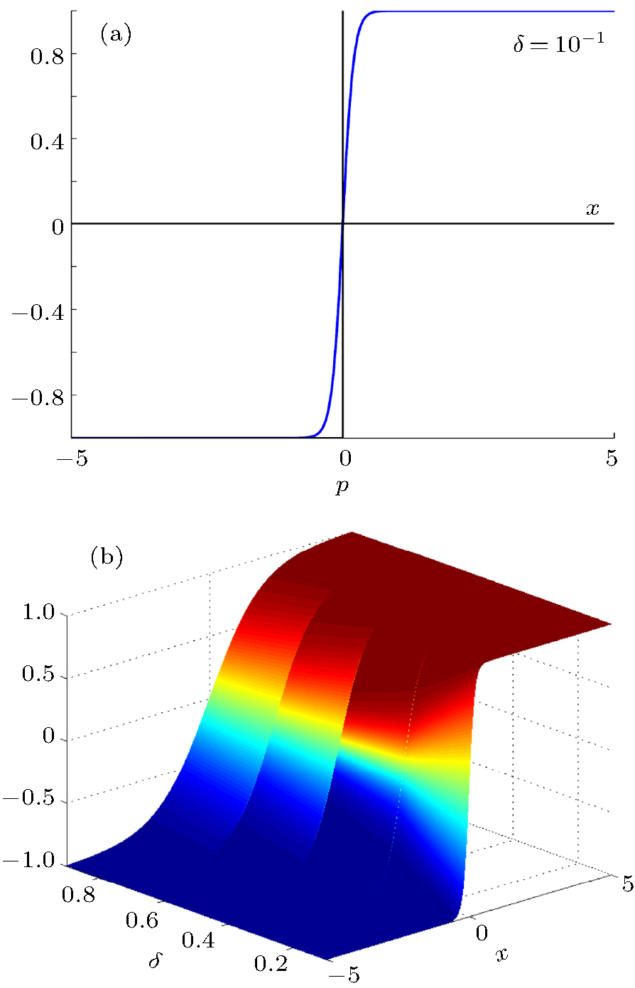	Fig. 3. (a) Graph of the sigmoid function for a large value of δ : δ = 10− 1; (b) graph of the sigmoid function depending on δ .

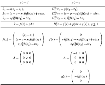
Using the sigmoid approximation (7), Chen’ s system (3) becomes

The cases studied in this paper are presented in Table 2.

Table 2.

Table 2.

Table 2. PWL Chen systems analyzed in this paper.

Table 2. PWL Chen systems analyzed in this paper.

Even for p : = a, the system does not belong to the class of systems modeled by the IVP (4), the PS algorithm still applies to this more general class of systems modeled by the following IVP (second column in Table 2)

where .

As is well known, in contrast with integer-order derivatives, if a function of class Cⁿ is periodic, its derivative in the sense of Caputo, Riemann– Liouville, and Grunwald– Letnikov, cannot be periodic with the same period (see e.g. Ref. [29]). However, in this paper we deal with numerical approaches of the continuous approximation of the PWL Chen system.

Next, we apply the PS algorithm to approximate stable cycles of Chen’ s PWL system of fractional-order (8), after it has been continuously approximated, for p : = d integer-order case, and p : = a integer and fractional-order cases. The case p : = a is an example of a new class of systems of integer and fractional-order where the PS algorithm still applies. For this purpose, we chose the sets 𝒫 and ℳ which generate the targeted values p*, after which the PS algorithm applies via the scheme (5). The targeted values for p* are chosen in the stable windows of BDs plotted in Fig. 2. For the phase plots, the transients have been omitted. To underline numerically and computationally the match between the two attractors, A* and A_p*, overplotted phase plots and time series have been used. The Hasudorff dimension, d_H (see Ref. [30] p. 114), is for all considered cases, of the order of 10^{− 3}, which indicates a good match between the two trajectories. In order to highlight the behavior characteristics of the utilized attractors, each illustrative case is accompanied by the underlying BD, such that the chaotic or regular motion character can be easily deduced.

Fig. 4.

	Figure Option ViewDownloadNew Window
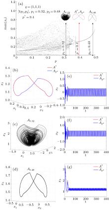
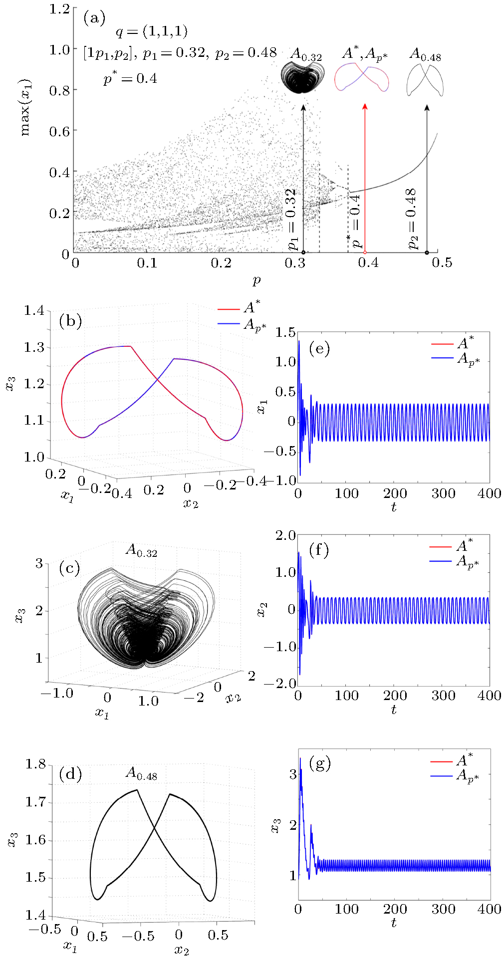	Fig. 4. PWL Chen’ s attractor A0.4, for p : = d, and q = (1, 1, 1), approximated with PS algorithm with the scheme [1p1, 1p2] with p1 = 0.32 and p2 = 0.48; (a) bifurcation diagrams; (b) overplotted attractors A* (red) and Ap* (blue); (c) attractor A0.32; (d) attractor A0.48; (e)– (g) overplotted time series corresponding to A* (red) and Ap* (blue).

All the computations were made in Matlab, using the RK4 and ABM methods for the integer-order and fractional-order systems respectively, with the integration step-size of the order of 10^{− 3}.

(i) p : = d

Commensurate case q = (1, 1, 1)

With a = 1.15, c = 2, and b = 0.15, the system behaves chaotically (see BD in Fig. 2(a)). Let us choose 𝒫 ₂ = {0.32, 0.48} (Fig. 4(a)) and ℳ = {1, 1} with the underlying scheme, [1p₁, 1p₂]. The switched attractor A* approximates the averaged attractor A_p* with p* given by Eq. (6): p* = 0.4. The match between both attractors can be seen in the overplotted phase plots in Fig. 4(b) and overplotted time series in Fig. 4(e)– 4(g). The underlying attractors A_0.32 and A_0.48 are chaotic and regular motion respectively (Figs. 4(c) and 4(d)).

(ii) p : = a

Since the case p : = d represents the case of the class of systems modeled by system (4), where the PS algorithm has been extensively studied in previous works, next we consider the case p : = a, which belongs to the class of systems modeled by system (9), and where the PS algorithm has not been applied yet. For b = 0.15, c = 2, and d = 0.1, as can be seen from the BD in Fig. 2(b), system dynamics are more complex than that for p : = d, presenting several direct and reverse period-doubling bifurcations. In this case, due to the term , the system is modeled by system (9). However, we will show that the PS algorithm still applies for this more general case.

a) Commensurate case q = (1, 1, 1)

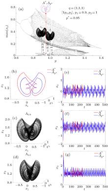
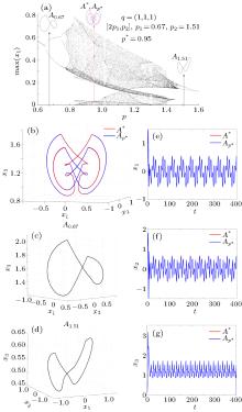
Choosing 𝒫 ₂ = {0.9, 1}, (see BD in Fig. 5(a)), with ℳ = {1, 1}, the relation (6) gives p* = 0.95, and with the scheme [1p₁, 1p₂] the PS algorithm generates the switched attractor A*, which approximates the stable cycle A_p* (see the phase plot in Fig. 5(b) and time series in Figs. 5(e)– 5(g)). Both underlying attractors A_1.9 and A_0.9 (Figs. 5(c) and 5(d)) are chaotic. Therefore, in this case, the PS algorithm acts as a control-like method (see Remark 2).

Fig. 5.

	Figure Option ViewDownloadNew Window
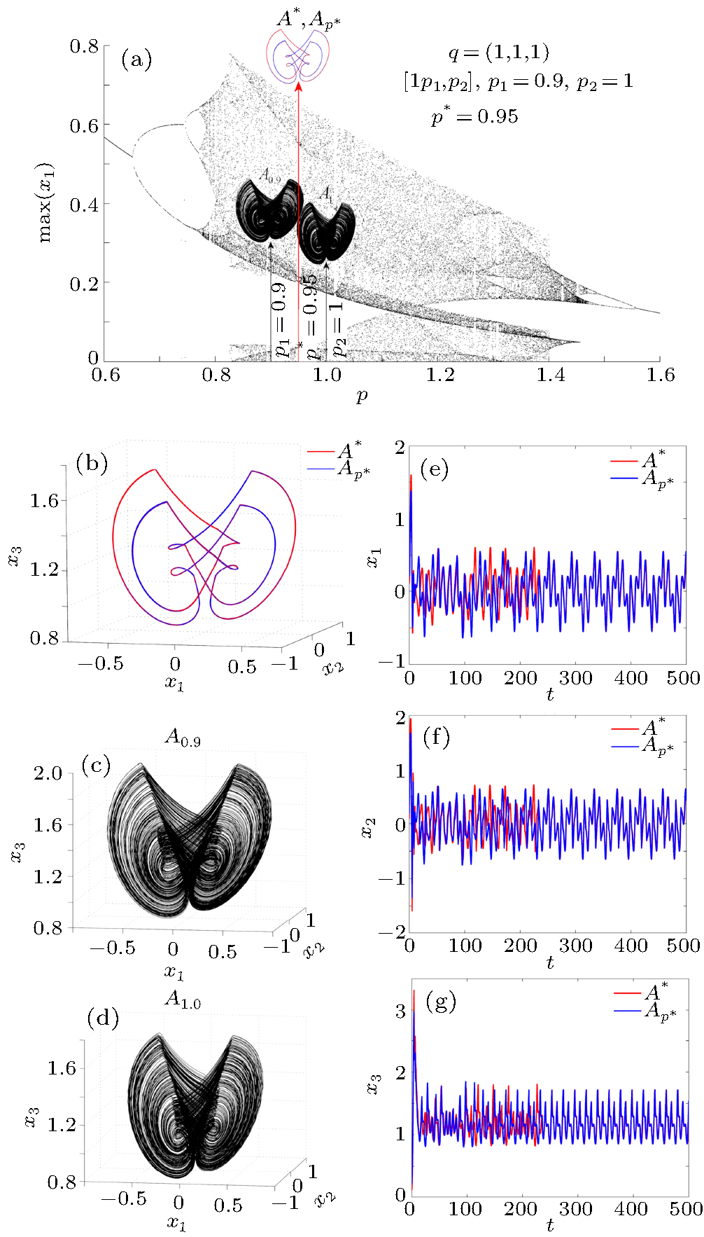	Fig. 5. PWL Chen’ s attractor A0.95, for p : = a, q = (1, 1, 1), approximated with PS algorithm with scheme [1p1, 1p2] with p1 = 0.9 and p2 = 1; (a) bifurcation diagram; (b) overplotted attractors A* (red) and Ap* (blue); (c) attractor A0.9; (d) attractor A1; (e)– (g) overplotted time series corresponding to A* (red) and Ap* (blue).

The non-uniqueness of solutions for p* in the relation (6), allows different ways to obtain some desired attractor A_p*. For example, the same attractor A_0.95 obtained above with the scheme [1p₁, 1p₂] (with values p₁ = 0.9 and p₂ = 1, situated in closed neighborhoods of p*), can be approximated by a switched attractor A* obtained with p values situated relatively distant from p*. For example, A_0.95 can be approximated with P_N = {0.67, 1.51} (Fig. 6(a)) and weights ℳ = {2, 1}, i.e. the scheme [2p₁, 1p₂]. Phase plots (Fig. 6(b)) and time series (Figs. 7(a)– 7(g)) reveal the approximation. This time, the stable cycle A* is obtained starting from parameter values which generate stable cycles (Figs. 6(c) and 6(d)).

Fig. 6.

	Figure Option ViewDownloadNew Window
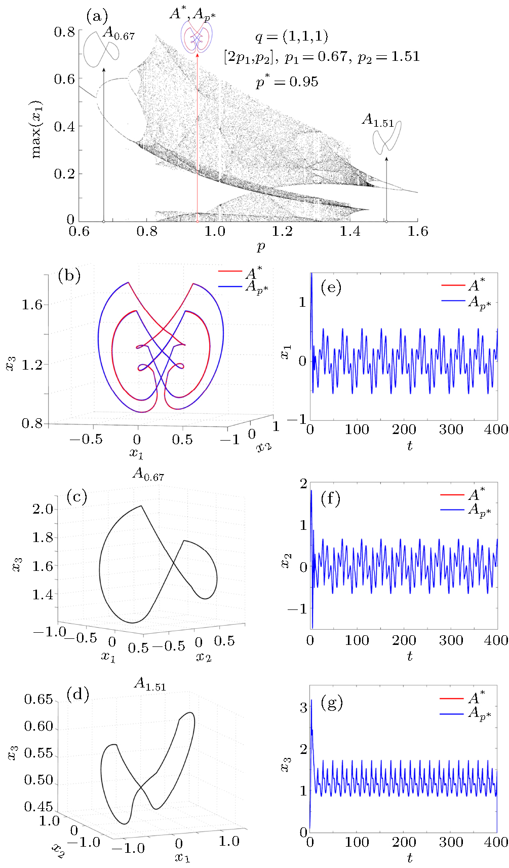	Fig. 6. PWL Chen’ s attractor A0.95, for p : = a, q = (1, 1, 1), approximated with PS algorithm with scheme [2p1, 1p2] with p1 = 0.67 and p2 = 1.51; (a) bifurcation diagram; (b) overplotted attractors A* (red) and Ap* (blue); (c) attractor A0.67; (d) attractor A1.51; (e)– (g) overplotted time series corresponding to A* (red) and Ap* (blue).

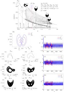
Also due to this same non-uniqueness, a set value p* can be obtained with N > 2 elements. For example p* = 0.95 can be obtained with 𝒫 ₆ = {0.6, 0.7, 0.8, 1.09, 1.32, 1.4} (see Fig. 7(a)) and ℳ = {1, 2, 2, 3, 1, 1}. By applying the PS algorithm with the underlying scheme [1p₁, 2p₂, 2p₃, 3p₄, 1p₅, 1p₆], one obtains again a good match between the two attractors A* and A_p* (Figs. 7(a)– 7(k)).

Fig. 7.

Figure Option ViewDownloadNew Window

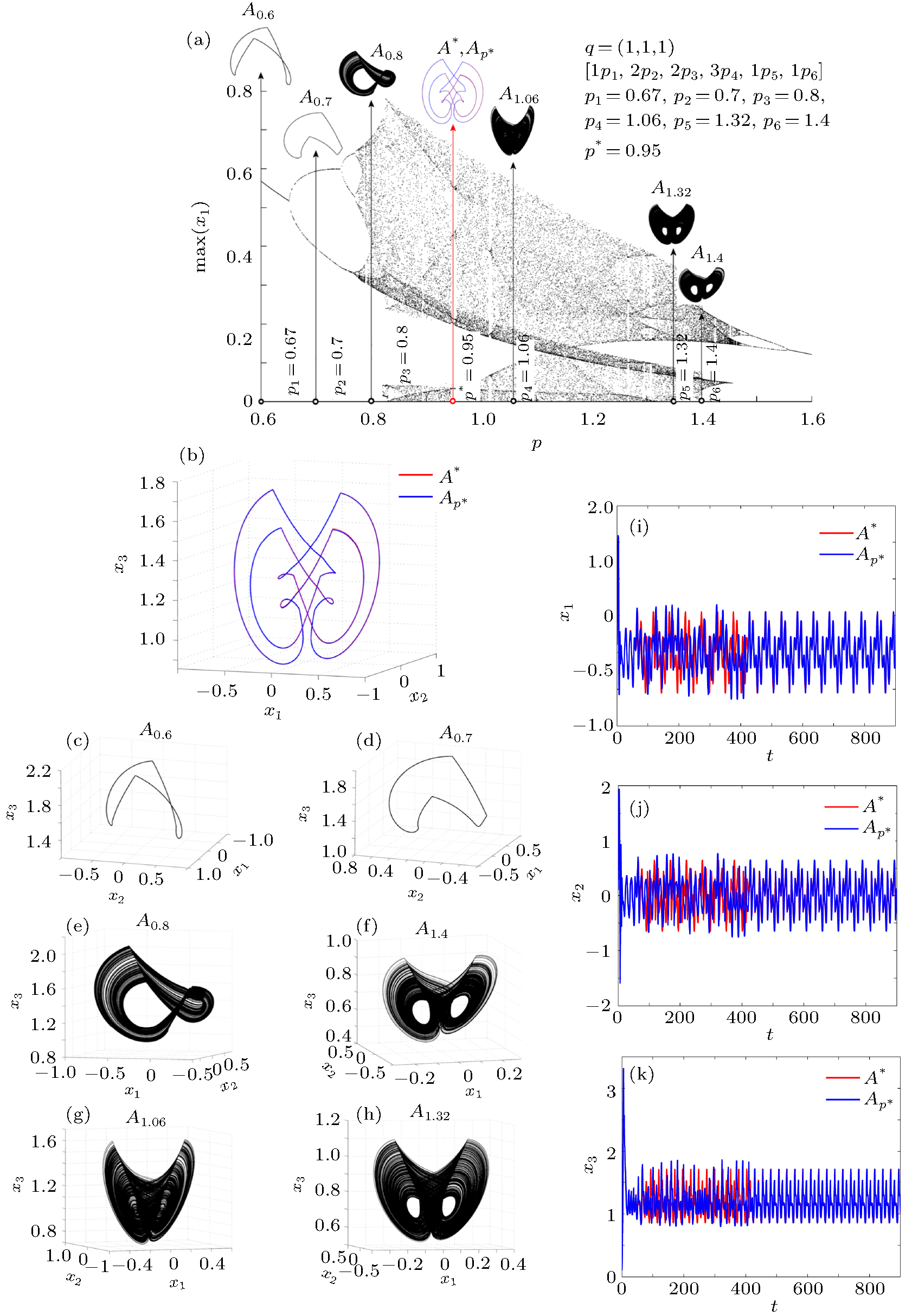Fig. 7. PWL Chen’ s attractor A0.95, for p : = a, q = (1, 1, 1), approximated with PS algorithm with the scheme [1p1, 2p2, 2p3, 3p4, 1p5, 1p6] with 𝒫 6 = {0.6, 0.7, 0.8, 1.09, 1.32, 1.4}; (a) bifurcation diagram; (b) overplotted attractors A* (red) and Ap* (blue); (c)– (h) attractors A0.6, A0.7, A0.8, A1.4, A1.06, and A1.32; (i)– (k) overplotted time series corresponding to A* (red) and Ap* (blue).

b) Incommensurate case q = (0.99, 0.98, 0.97)

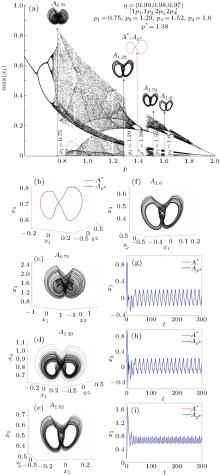
With 𝒫 ₄ = {0.75, 1.29, 1.52, 1.6, 1.38} (see the bifurcation diagram in Fig. 8(a)) and ℳ = {1, 1, 2, 2}, the PS scheme [1p₁, 1p₂, 2p₃, 2p₄] generates the attractor A*, which approximates A_p* with p*= 1.38. The match between the two attractors is revealed in Fig. 8(a)– 8(i). Again the PS algorithm acts like a control-like method.

Fig. 8.

	Figure Option ViewDownloadNew Window
	Fig. 8. PWL Chen’ s attractor A1.38, for p : = a, q = (0.99, 0.98, 0.97), approximated with PS algorithm with the scheme [1p1, 1p2, 2p3, 2p4] with 𝒫 4 = {0.75, 1.29, 1.52, 1.6}; (a) bifurcation diagram; (b) overplotted attractors A* (red) and Ap* (blue); (c)– (f) attractors A0.75, A1.29, A1.52, A1.6; (g)– (i) overplotted time series corresponding to A* (red) and Ap* (blue).

In this paper we present a new version of Chen’ s system: the PWL Chen system of fractional-order, revealing interesting new dynamical characteristics, including the coexistence of chaotic and regular motions. To numerically cope with this system, we first must make a continuous approximation of the discontinuities by using an algorithm based on Filippov’ s regularization and also by applying Cellina’ s Theorem. The approximation is implemented via the sigmoid function (7).

We show that the stable attractors can be numerically approximated with the PS algorithm by starting from a set of parameter values which are periodically switched while the underlying IVP is numerically integrated. Results are robust across a range of moderate small step sizes.

We note that the case p : = a allowed us to verify that the PS algorithm applies also to a new general class of systems modeled by system (9).

One of the open and most intriguing problems is revealed by the following question: Even though the PWL equation (3) and the continuous equation (8) are equivalent in the sense of numerical approximation, with some experimental (circuitry) implementations of both systems, will they reveal the same behavior? A positive answer to this question will be useful to underline the importance of this approach of PWL systems.

Also, the convergence proof of the PS algorithm for other larger classes of IVPs remains the subject of future works.