It is well known that the study of the motion of charged particles under a magnetic field is an essential topic in both macroscopic and microscopic physics. In particular, a number of distinguished quantum mechanical phenomena, such as the Aharonov– Bohm (AB) oscillation and the fractional quantum Hall effect (FQHE), are caused by the magnetic gauge field.^{[1– 3]} After the experimental realization of the condensation of neutral atoms with nonzero spin, ^[4] a great interest is to create a light-induced gauge vector field to achieve the spin– orbit coupling (SOC) so that various magnetic– electronic phenomena of charged particles occurring in condense matters can be copied into the world of condensates of neutral atoms.^{[5– 9]} Since 2005 there have been proposals by the theorists for producing the light-induced gauge vector field for the condensates with multi-component neutral cold atoms.^{[10– 15]} The first experimental realization of the SOC in condensates was implemented in 2009 by dressing the cold atoms with two counter propagating polarized laser beams.^{[16, 17]} This technique opened a new perspective in the field of BEC, and more and more experimental^{[18– 21]} and theoretical^{[22– 24]} results have been reported. It was found that the total magnetization (or spin-polarizability, which measures the difference of the densities of the spin-components) varies with time. It implies the existence of spin-currents.^{[12, 16, 22]} Besides, the collective-mode dynamics has been studied, the spatial motions along different directions could be correlated (say, a dipole mode might induce a breathing mode in its perpendicular plane).^[24] The instability caused by the collective mode has also been studied.^[23]

On the other hand it is now possible to trap a condensate in ring geometry. Long-lived rotational superflows have been induced in this kind of system.^{[20, 25– 33]} The creation of the spin-currents of two-component condensates on a ring, due to the introduction of the laser beams, has been experimentally realized.^[20] It was found that the stability depends strongly on the initial ratio of the two components.^[20] However, the oscillation of the spin-currents on the ring has not yet been observed.

Obviously, the study of the cold spin-currents (i.e., the current of each spin-component) caused by the SOC is just beginning. It is expected that the oscillation of the spin-currents might also emerge in the ring geometry (because a circular motion is equivalent to a linear motion with a periodic boundary condition). To confirm this suggestion, a one-dimensional model of the two-component condensates on a ring under SOC is adopted in this paper. The aim is to clarify from the theoretical aspect how the details of oscillation (the period and amplitude) depend on the parameters of the laser beams. We believe that the interaction might not be crucial. Therefore, the interaction is ignored at first so as to emphasize the decisive role of the laser beams. Then, the effect of the interaction is evaluated via a two-body system.

Let the quasi-spin ŝ be introduced to describe the two components of an atom as usual. The atomic state with s_z = 1/2 (− 1/2) is named the up- (down-)state. When two counter-propagating and polarized laser beams are applied, due to the SOC, the two components of atoms might move towards opposite directions along the beams and can transform to each other via a spin-flip. When the interaction is ignored, the Hamiltonian is just H = ∑ _iĥ _i, where ĥ _i is for the i-th particle. Disregarding the subscript i,

where θ is the azimuthal angle along the ring.^[9] The unit of energy is hereafter E_unit ≡ ħ ²/(2mR²), where m is the mass of an atom, R is the radius of the ring. β ≡ k₀R, where 2k₀ is the momentum transfer caused by the two lasers. γ ≡ Ω /2E_unit, where Ω /2 is the strength of Raman coupling causing the spin-flips accompanied by the momentum transfer. Let ε _split be the Zeeman energy difference between the two spin-states, and ω _δ is the frequency difference between the two laser beams. We define the Raman detuning δ ≡ (ε _split − ħ ω _δ )/(2E_unit). In addition to γ , δ is an important quantity because it can be tuned so that the related process could be energy-adapted (see below). Note that, due to the ring geometry, 2β must be an integer. It implies that the transfer of momentum will be suppressed unless the transfer is close to a specific set of values depending on R. Thus, an additional constraint is required under the ring geometry.

To illustrate the connection with conventional SO coupling, we define a U-transformation so that the up-state (down-state) is multiplied by a factor e^{iβ θ} (e^{− iβ θ} ). Then, by introducing the Pauli matrices σ _z and σ _x, Uĥ U^{− 1} can be written in a more familiar form as^{[9, 12, 16, 34, 35]}

where σ _I is just a unit matrix with rank 2. ĥ has two groups of eigenstates, they can be written as^{[16, 34, 35]}

where

k is an integer (half-integer) when β is an integer (half-integer),

s_γ is the sign of γ , , and ρ _k ranges from − π /2 → π /2. One can see that the eigenstates have two notable features:

The eigenenergies of are . Obviously, .

The time-dependent solution ψ (θ , t) of the single-particle Schrö dinger equation starting from an initial state ψ _init can be formally written as

where τ ≡ tE_unit/ħ (for ⁸⁷Rb and R = 12 μ m as given in Ref. [20], t = 0.398 τ s), λ = ± , k runs over the (half-) integers when β is the (half-) integer.

In the experiment reported in Ref. [21] a strong oscillation of the magnetization induced by a sudden change of the laser field was reported. It is assumed that a set of parameters β , γ ₁, and δ ₁ (the first set) are given initially, and the initial state is just the ground state (g.s.) of ĥ as , where q depends on the three parameters so that the associated energy is the lowest. The superscript in implies that it is obtained from the first set of parameters. Then, γ ₁ and δ ₁ are suddenly changed to γ ₂ and δ ₂ (the second set). Accordingly, we have a new Hamiltonian and a new set of eigenstates. With them ψ (θ , t) becomes

where

and

Where and are obtained from γ ₂ and δ ₂. From ψ (θ , t), we know that the two components of the g.s., φ _{q− β , ↑} and φ _{q− β , ↑} , remain unchanged. However, the coefficients of composition are not more constants but oscillate with τ .

Let the time-dependent densities of the up- and down-components be defined from the identity ψ ⁺ (θ , t)ψ (θ , t) ≡ n_↑ (θ , τ )+ n_↓ (θ , τ ). Then, we have

The magnetization (or spin-polarization) is defined as P_z = (n_↑ − n_↓ )/(n_↑ + n_↓ ). We have

This formula gives a clear picture of a harmonic θ -independent oscillation with a period and an amplitude .

Based on the second set of parameters let us define the energy difference of the two components as

Then, the frequency of oscillation . This formula demonstrates that both the strength of the Raman coupling and the energy difference are crucial. A larger | γ ₂| leads always to a higher frequency ≥ | γ ₂| /π . This frequency can be further tuned by varying δ ₂ around 2qβ . In particular, when δ ₂ is tuned so that is zero, 1/τ _p will arrive at its conditional minimum | γ ₂| /π . Since depends on q but not on the other details of the initial state, 1/τ _p depends essentially on the second set of parameters when q is given.

On the other hand, the amplitude A_amp depends on both sets of parameters explicitly. When the first set of parameter has been given so that is fixed, A_amp will arrive at its conditional maximum at a specific value of , namely, (if γ ₂ < 0 and ), or (if γ ₂ > 0 and ), or (if γ ₂ < 0 and ), or (if γ ₂ > 0 and ), or (if γ ₂ < 0 and ), or (if γ ₂ > 0 and ). It implies that, no matter how the first set of parameters are, one can tune the second set so that the amplitude is conditionally maximized, namely, . In particular, when γ ₁ = 0, we have or 0. In this case, if γ ₂ ≠ 0 and δ ₂ are tuned so that , then and the amplitude would arrive at its absolute maximum, namely, A_amp = 2. Note that the condition or 0 implies that the initial state is pure without mixing (namely, either ψ _init = φ _{q − β , ↑} or φ _{q+ β , ↓} ), while the fact A_amp = 2 implies a complete transformation of the two components (namely, from a pure up-state to a pure down-state, or vice versa). Therefore, γ ₁ = 0 is required so that the maximal amplitude could be realized. On the other hand, in any cases, when γ ₂ and γ ₁ have the same sign and , or γ ₂ and γ ₁ have opposite signs and , A_amp → 0 and the oscillation damps. This is obvious from the expression of A_amp.

In addition to the densities, one can further define the current based on the equation of continuity as

From this definition we found that the current j = j_↑ + j_↓ in which j_↑ ≡ j_unitn_↑ (q − β ) is the current of the up-component and is named up-current, while j_↓ ≡ j_unitn_↓ (q + β ) is the down-current, where the unit is j_unit = ħ /(mR²).^[23] The currents are also oscillating with the same period , and they are also θ -independent. Obviously, when | β | > | q| , j_↑ and j_↓ will have different signs. Therefore, counter propagating currents emerge. This is a distinguished feature.

The above formulae arise from a single-particle Hamiltonian. For N-particle systems, when all the particles fall into the same state ψ _gs initially and the interaction is ignored, it is straightforward to prove that the above formulae hold also.

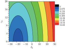
To give numerical results, the radius is given at R = 12 μ m in this paper. A contour diagram for the frequency 1/τ _p versus γ ₂ and δ ₂ is shown in Fig. 1. Where the minimum is located at γ ₂ = 0 and (namely, δ ₂ = 2qβ = − 18), at which the oscillation vanishes.

Fig. 1.

	Figure Option ViewDownloadNew Window
	Fig. 1. The frequency 1/τ p versus δ 2 and γ 2. The oscillation is caused by a sudden change in γ and δ . β = 3 and q = − 3 are given. The values of the contours are in an arithmetic series. The contour closest to the right side has the largest value 1/τ p = 14.5.

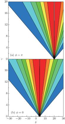
Two contour diagrams for A_amp versus γ ₂ and δ ₂ with γ ₁ and δ ₁ being fixed are shown in Fig. 2, where all the contours appear as straight lines. This arises from the fact that can be rewritten as a function of together with the two signs of γ ₂ and δ ₂– 2qβ (it implies that a given is associated with a straight line on the δ ₂– γ ₂ plane). In Figs. 2(a) [2(b)] the given values of β , γ ₁, and δ ₁ lead to q = − 3 [3] and . According to the discussion given previously and when γ ₂ > 0, the maximum of A_amp should appear when in Fig. 2(a), and in Fig. 2(b). This maximum is associated with the straight dotted line marked in the figure. (Incidentally, if , then the associated straight line would be vertical. Since the two dotted lines have their close to π /4, they are nearly vertical.) Whereas when , the associated straight line is marked by a solid line in the figure (where the small circle marks the place that γ ₂ = γ ₁, and δ ₂ = δ ₁). Three notable features are evoked:

Fig. 2.

Figure Option ViewDownloadNew Window

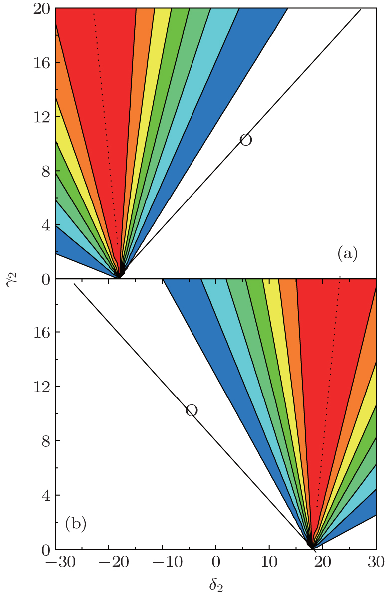Fig. 2. The amplitude Aamp versus δ 2 and γ 2. β = 3, γ 1 = 10, and δ 1 = 5 [− 5], are given in panel (a) [(b)]. Accordingly, q = − 3 [3] in panel (a) [b]. The oscillation is caused by a sudden change fromγ 1 to γ 2 and δ 1 to δ 2. The dotted line marks the locations where (a), or (b). Thus this line marks the conditional maximum of in both panels (a) and (b), which is the largest value in each panel. The contours going away from this line are in an arithmetic series and decrease to zero. The black small circle marks the location where δ 2 = δ 1 and γ 2 = γ 1. The solid line passing through the circle marks the locations where and accordingly Aamp = 0.

Recently, the initial state was prepared in a superposition state in an experiment of cold atoms with the ring geometry.^[20] In this experiment an additional radio frequency field was used for preparing the initial state

where ϕ determines the initial ratio of the two components and is tunable (0 ≤ ϕ ≤ π ). q is a tunable integer and marks the initial angular momentum of the particle. In this case we have the set of parameters ϕ , q, β , γ , and δ . The corresponding time-dependent solution is

where

and

Accordingly, we can obtain the up- and down-densities n_↑ (θ , τ ) and n_↑ (θ , τ ) given in Appendix A. From them the magnetization P_z can be obtained. It is apparent that, when ϕ = π or 0 (i.e., ψ _init is a pure up-state or down-state) the magnetization has a very simple form as

if ϕ = π , or

if ϕ = 0.

These formulae also give a clear picture of harmonic oscillation, but the periods are different for the two cases of ϕ .

When ϕ = π , τ _p = π /a_{q+ β} . If δ is tuned so that δ = 2(q + β )β ≡ δ ₀, the frequency will be minimized, namely, . When δ goes away from δ ₀, the frequency increases. The amplitude A_amp = 1 − cos(4ρ _{q+ β} ). Obviously, when δ = δ ₀, we have ρ _{q+ β} = ± π /4, and the amplitude would arrive at its maximum, namely, (A_amp)_max = 2. Furthermore, when γ → ± 0, one can prove that ρ _{q+ β} will tend to 0 or ± π /2. In any of these cases A_amp = 0 and the oscillation disappears. This implies that γ is the source of the oscillation.

When ϕ = 0, the discussion in the preceding paragraph holds also, except that q + β should be changed to q − β , and δ ₀ should be replaced by 2(q − β )β . An example of A_amp is shown in Fig. 3. Figure 3 is of a similar form to Fig. 2 (all the contours are straight lines that converge to a point with γ = 0) except that the dotted line in Fig. 3 is exactly vertical.

Fig. 3.

	Figure Option ViewDownloadNew Window
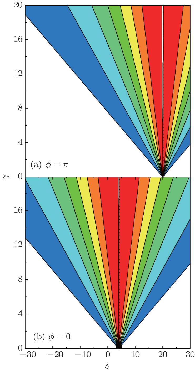	Fig. 3. The amplitude Aamp versus δ and γ for the case that the initial state is a superposition state. q = 3 and β = 2 are assumed. ϕ = π [0] are given in panel (a) [(b)]. The dotted line marks the maximum ofAamp = 2. The locations with γ = 0 have Aamp = 0.

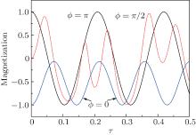
When ϕ is neither π nor 0, the oscillation is no longer harmonic. In particular, both the up- and down-densities depend on θ (refer to Appendix A). It implies that the densities are not uniform on the ring as before. Consequently, stripes emerge along the ring, and the stripes move with time. An example of the evolution of P_z is shown in Fig. 4, where the relation δ = 2(q + β )β holds. Accordingly, the curve with ϕ = π has the maximized A_amp = 2 and a minimized frequency. Whereas the curve with ϕ = 0 has a smaller A_amp and a larger frequency. For ϕ = π /2, the anharmonic oscillation is clearly shown.

Fig. 4.

	Figure Option ViewDownloadNew Window
	Fig. 4. The magnetization Pz versus τ observed at θ = 0 for the case that the initial state is a superposition state with a ϕ marked by the curve. q = 3, β = 2, γ = 15, and δ = 20 are assumed. When ϕ = π or 0 the oscillation is harmonic. Otherwise, it is not.

An example of the up-density versus θ with ϕ = π /2 is shown in Fig. 5, where the stripes emerge along the ring. Note that two waves φ _{q, ↑} and φ _{q− 2β , ↑} are contained in the up-component, and φ _{q, ↓} and φ _{q+ 2β , ↓} in the down-component. The stripes arise from the interference of these waves. Note that one of these waves contains an additional factor e^{∓ i2β θ} . Accordingly, the stripes appear periodically with θ as shown in Fig. 5 and the number of peaks (valleys) in the domain (0, 2π ) is 2β (say, the number is four in Fig. 5, where β = 2). The locations of the peaks of the stripes move with time, the magnitudes of the peaks also change with time.

Fig. 5.

Figure Option ViewDownloadNew Window

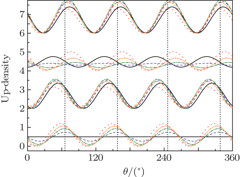Fig. 5. Up-density n↑ versus θ with ϕ = π /2. The densities are given by 20 curves for a sequence of τ . Starting from τ = 0, in each step τ is increased by 1/40. The 20 curves in the sequence are divided into 4 groups. The n↑ of each group has been shifted up by two relative to its preceding group, for a clearer perspective. The five n↑ in each group are plotted in solid, dash, dash– dot, dash– dot– dot, and dot lines, respectively, according to the time-sequence (τ = 0 is the horizontal solid line in the lowest group). The parameters are q = 1, β = 2, γ = 10, and δ = 1. The vertical dotted lines are also for guiding the eyes.

As before, when all the particles are given in the same ψ _init initially and the interaction is ignored, the above formulae and discussion hold also for N-particle systems.

When the interaction is taken into account, the total Hamiltonian is H = ∑ _iĥ _i + ∑ _{i< j}V_ij, where V_ij = gδ (θ _i − θ _j), g = g_{↑ ↑} (if both atoms are up), g_{↓ ↓} (both down), or g_{↑ ↓} (one up and one down). In order to evaluate the effect of interaction in the simplest way, we study a two-body system. Firstly, a set of single particle states

where , and − k_max ≤ k ≤ k_max, are adopted. Accordingly, we have 2(2k_max + 1) single particle states, and they are renamed as φ _j ≡ φ _{kjμ j}. Based on φ _j a set of basis functions for the two-body system Φ _i = S̃ [φ _j(1)φ _j′ (2)] are defined, where S̃ is for the symmetrization and normalization, and j ≥ j′ .

Note that the strength of a pair of realistic Rb atoms is g_Rb = 7.79 × 10^{− 12} Hz· cm³ (the differences in the strengths between the up– up, up– down, and down– down pairs are very small and are therefore disregarded). Since the atoms in related experiments are not distributed exactly on a one-dimensional ring but in a domain surrounding the ring, the effect of the diffused distribution should be considered. Hence, for each φ _kμ we define its three-dimensional (3D) counterpart

where the Gaussian function e^{− (r/r_w)2} describes the diffused distribution and r_w measures the width of the distribution. With we define an effective strength g_eff so that for any pair of matrix elements

Then, we have

which is the effective strength adopted in our calculation.

It is assumed that both atoms are given at the same superposition state with ϕ = π or 0 initially. When the Hamiltonian is diagonalized in the space expanded by Φ _i, the eigenenergies E_l and eigenstates Ψ _l ≡ ∑ _iC_liΦ _i can be obtained, and the time-dependent state is

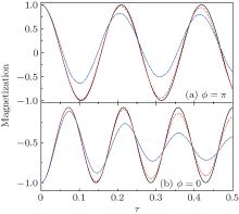
where Ψ _init = ψ _init(1)ψ _init(2). From Ψ (θ , t) the densities and P_z(t) can be calculated. An example with k_max = 14 is shown in Fig. 6 where the strength g is given at three values. When k_max is changed from 14 to 12, there are no explicit changes in the pattern. It implies that the choice k_max = 14 is sufficient in qualitative sense.

Fig. 6.

	Figure Option ViewDownloadNew Window
	Fig. 6. Pz of a two-body system of Rb atoms versus τ with interaction Vij = gδ (θ i − θ j), g = 0 (solid), 100geff (dash), and 2000geff (dash– dot). The initial state has ϕ = π (a) and ϕ = 0 (b). . The other parameters are the same as those in Fig. 4.

In Fig. 6 the curves “ 1” and “ 2” overlap approximately. It implies that the effect of interaction with a g ≤ 100g_eff is very small. However, when g = 2000g_eff, the amplitude decreases with time explicitly as shown by the dash– dot curve, while the period remains nearly unchanged. Note that, based on the Gross– Pitaevskii equation, the effect of the combined interaction imposing on a single particle from the other N − 1 particles is similar to an appropriate strengthening of the strength of the atom– atom interaction. Thus the explicit dampening that happens when g = 2000g_eff implies that, for an N-body system with a larger N, the dampening would actually occur. This is a topic to be clarified further. In fact, the dampening of the oscillation has already been observed in all related existing experiments.^{[16, 21]}

In summary, the oscillation of the cold atoms under the SOC and constrained on a ring has been studied analytically without taking the interaction into account. Then, the effect of the interaction is evaluated numerically via a two-body system. Two cases, namely, the evolution that starts from a g.s. and is induced by a sudden change of the laser field, and the evolution that starts from a superposition state, are involved. The emphasis is placed on clarifying the relation between the parameters of the laser beams and the period and amplitude of the oscillation. This is achieved by giving a set of formulae so that the relation can be understood analytically. The conditions that the frequency and/or the amplitude can be maximized or minimized have been predicted. To realize the mutual-transformation of the two components, not only the strength of the Raman coupling γ is important, the energy difference between the two components is also important which can be tuned by δ (this is similar to the case of a resonance). The frequency of oscillation will increase with γ in general, while the amplitude depends on the inter-relation of γ and δ . When (δ , γ ) vary along a specific straight line on the δ – γ plane, the amplitude may increase, decrease, or even remain unchanged depending on the slope of the line. This is a common feature for the first case and for the second case with ϕ = π or 0, whereas when ϕ ≠ π and 0, movable stripes will emerge on the ring. Experimental confirmation of the regularity unveiled in this paper and the predicted phenomena is expected.